Computer Network

Welcome to the student resources for the Computer Networking: A Top-Down Approach Sixth Edition Companion Website.

INTERACTIVE END-OF-CHAPTER EXERCISES, Supplement to Computer Networking: A Top Down Approach 8th Edition

Interactive Animations

The Illustrated QUIC Connection: Every Byte Explained（QUIC 协议图解）

Baida | HTTPS explained with carrier pigeons

Computer Network and Internet

Network Edge

因特网是世界范围的计算机网络。传统的桌面 PC、Linux 工作站、服务器，以及新兴的手机、家用电器、可穿戴设备等正在与因特网相连。这些设备被称为主机 (host)，主机又可分为两类：客户端和服务器；因主机运行在网络边缘 (network edge)，故又称为端系统 (end system)。

Access network—the network that physically connects an end system to the first router.

• 家庭入网过去用的是 DSL (Digital Subscriber Line)，DSL modem 得到数字信息后将其转换为高频信号，通过电话线（即双绞铜线）与电话公司的 DSLAM 交换数据，并在那里被转换回数字形式。电话线通过“频分复用技术”形成了双向电话信道（0 - 4kHz）、中速上行信道（4kHz - 50kHz）、高速下行信道（50kHz - 1MHz）。使得电话呼叫和因特网连接能同时进行。
• 另一种家庭入网是同轴电缆 (cable) 接入，利用了有线电视公司的基础设施。家庭先通过同轴电缆接入到地区的光纤节点，再通过光纤连接到有线电视公司。这种入网要用到 cable modem，同 DSL modem 一样将信号进行数模转换。
• 现在更多的家庭享受到了光纤入户 (Fiber To The Home, FTTH)，用户在家中将无线路由器与 ONT (Optical Network Terminator) 相连，多个家庭的 ONT 通过光纤连接到临近的分配器 (splitter)，再通过一根共享的光纤连接到本地中心局的 OLT (Optical Line Terminator)。OLT 提供了光信号和电信号之间的转换。

Network Core

Packet Switching

网络核心是由通信链路 (communication link) 和分组交换机 (packet switch) 构成的网状网络。端系统彼此交换报文 (message)。长的报文被划分成分组 (packet)，分组通过网络核心传送。

通信链路由不同的物理媒体组成，包括同轴电缆、双绞铜线、光纤、无线电频谱等。链路的传输速率以 bit/s 度量。假设链路的传输速率是 R bits/s，经过一条链路发送 L bits 的 packet，传输时间应为 L/R 秒。

Packet switch 最著名的两种类型是路由器 (router) 和链路层交换机 (link-layer switch)。

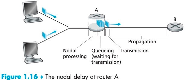
Packet 在传输的路径上的每个节点都要经历几种不同类型的时延。

节点处理时延 (nodal processing delay)：检查 packet 的头部并决定将该 packet 导向何处。

排队时延 (queuing delay)：对于每一条连接到 packet switch 上的链路，都有一个对应的输出缓存 (output buffer)，它用于存储准备发往那条链路的 packet。如果该链路正忙于传输，则到达路由器的 packet 必须在输出缓存中等待，这就造成了排队时延。如果输出缓存已满，那么在新的 packet 到达时就会有 packet 被丢弃，造成丢包。

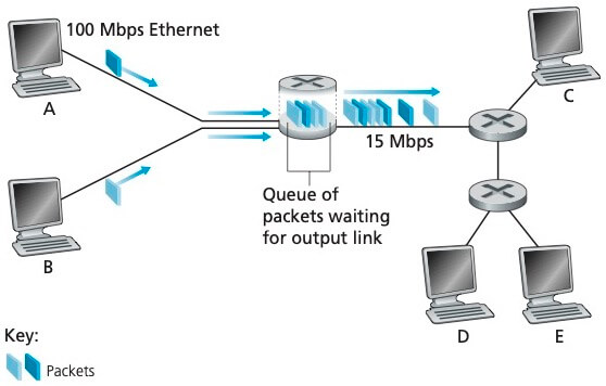
传输时延 (transmission delay)：L/R，这是将一个 packet 的所有比特推向链路的时间，传输时延的原因是存储转发机制。

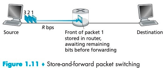
多数 packet switch 在链路的输入端使用存储转发传输 (store-and-forward transmission)，这是指 packet switch 在开始向输出链路传输 packet 的第一个比特之前，必须收到整个 packet。

为了理解这一机制，考虑两个端系统经一台路由器连接构成的简单网络，Source 在时刻 0 开始传输，经过 L/R 秒，路由器接受到整个 packet，并且开始向出链路传输，在时刻 2L/R 整个 packet 到达目的地，所以总时延是 2L/R。如果 packet switch 不使用存储转发机制，而是每到达一个比特就直接转发，那么总时延将会是 L/R。

一般地，通过由 N 条速率均为 R 的链路组成的路径（代表有 N - 1 台路由器），端到端的存储转发时延是 d = N * L / R。

传播时延 (propagation delay)：一旦一个比特被推向链路，它就会向下一个节点传播，这是一个比特从路由器 A 的出口到路由器 B 的入口所需要的时间。传播速率取决于该链路的物理媒体。

下面一张图概括了路由器 A 的节点总时延 (total nodal delay)：

Circuit Switching

Circuit Switching 必须在发送方和接收方之间建立一条连接，该连接被称为一条电路 (circuit)，它路径上的交换机都要为该连接维护必要的状态。Circuit 预留了恒定的传输速率，以确保发送方能够以恒定速率向接收方传送数据。（类比固定电话之间的通话）

与之相反，packet switching 不预留任何链路资源，因特网尽最大努力交付 packet 但不做任何保证。（类比微信语音通话）

Circuit Switching 需要预先分配资源，已分配而没有用上的链路时间就被浪费掉了；Packet Switching 则可以按需共享链路传输能力。今天的电信网络正在朝 Packet switching 发展，特别是，电话网经常在昂贵的海外电话部分使用 Packet Switching。

Internet Service Provider

端系统要通过 ISP (Internet Service Provider) 接入因特网。Access ISPs 的类型多种多样，包括住宅 ISP、公司 ISP、大学 ISP、咖啡厅或医院等公共场所的 ISP……

在中国，每个城市有 Access ISPs，它们与省级 ISP 连接，再与国家级 ISP 连接，最终与 tier-1 ISP 连接；在此基础上，再加上 PoPs (Point of Presence)、multi-homing、peering、IXPs (Internet exchange points)、内容提供商网络 (content provider network) ，构成了今天的因特网结构。

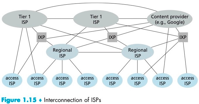
总之，今天的因特网是一个网络的网络，结构非常复杂，由十多个 tier-1 ISP 和数十万个较低层 ISP 组成。用户和内容提供商是较低层 ISP 的客户，低层 ISP 是高层 ISP 的客户。例如谷歌通过创建自己的网络和数据中心，直接在可能的地方与低层 ISP 互联。

Protocol Layers

网络设计者以分层的方式组织协议、并实现这些协议的网络硬件和软件。一个 layer 会使用它下层的服务，并同时向上层提供服务 (service model)。

各层的所有协议被称为协议栈 (protocol stack)，因特网的协议栈由 5 个层次组成：物理层、链路层、网络层、运输层、应用层。

传输层负责进程到进程的传送；网络层负责主机到主机的传送；链路层负责将帧从一个节点移动到邻近的下一个节点；物理层负责将帧中的每一个比特从一个节点移动到下一个节点。

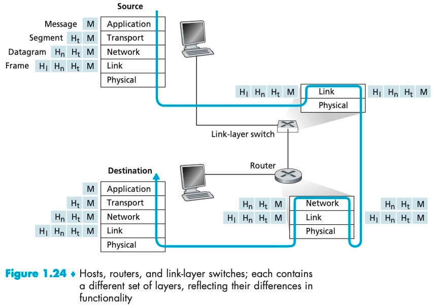
上图显示了这样一条路径：数据从源的协议栈一路向下、经过中间的链路层交换机和路由器的协议栈上上下下、最后向上到达目的地的协议栈。注意，路由器实现了第一层到第三层协议，而链路层交换机只实现了前二层。这意味着路由器能够实现 IP 协议，但链路层交换机不能，因此它不能识别 IP 地址，但它能够识别第二层地址如 Ethernet 地址。如上图所示，packet 到达每一层，都会被附加上该层的首部字段（用字母 H 表示），首部字段会在之后被相应的层使用。

Application Layer

在同一个端系统上的进程，它们使用 IPC 相互通信，规则由操作系统确定；在两个不同端系统上的进程，通过跨越计算机网络交换 message 而相互通信。

不管是 client-server architecture 还是 P2P architecture，对每对通信进程，我们把主动发起通信方称为客户端，被动等待联系方称为服务器。在 P2P architecture 中，一个进程既能够是客户端又能够是服务器。

进程通过一个称为 socket 的软件接口发送和接收 message。

在因特网中，目的地主机由 IP 地址标识；接收进程由端口号标识。

开发一个应用时，必须选择一种运输层协议，如何选择呢？大体从可靠数据传输、吞吐量、时效性和安全性几个方面考虑。如电子邮件、Web 文档这类应用，必须保证可靠数据传输（不能丢失数据）、对吞吐量无要求、对响应时间不敏感；流媒体、视频通话、游戏等应用，则可以容忍丢包、但对带宽有要求、对响应时间敏感。

TCP 为应用层提供了面向连接的、可靠数据传输服务，还具有拥塞控制机制；UDP 是一种“仅提供最小服务”的传输层协议，它不提供可靠数据传输服务，不保证 message 能到达、能有序到达接收进程。

TCP 和 UDP 本身都没有提供安全性相关的服务，但 TCP 在应用层可以用 SSL 来提供安全服务。除了可靠数据传输和安全性，目前的因特网运输协议并不能提供吞吐量和时效性的保证。

The Web and HTTP

The HyperText Transfer Protocol (HTTP), the Web’s application-layer protocol, is at the heart of the Web.

A Web page (also called a document) consists of objects. An object is simply a file—such as an HTML file, a JPEG image, a Javascrpt file, or a video clip—that is addressable by a single URL. Most Web pages consist of a base HTML file and several referenced objects.

HTTP defines how Web clients (Web browsers) request Web pages from Web servers (e.g. Apache) and how servers transfer Web pages to clients.

It is important to note that the server sends requested files to clients without storing any state information about the client. If a particular client asks for the same object twice in a period of a few seconds, the server does not respond by saying that it just served the object to the client; instead, the server resends the object, as it has completely forgotten what it did earlier. Because an HTTP server maintains no information about the clients, HTTP is said to be a stateless protocol.

为什么说 HTTP 是无状态的？原因是 HTTP 协议不要求服务器保存用户的任何信息和状态。对于每个请求，服务端都把它当作新的、陌生的请求来处理。虽然协议本身无状态，但可以通过使用 cookie 来追踪用户的信息。

HTTP 在默认方式下使用持续连接 (persistent connection)，意味着客户端和服务器在一个长的时间范围内通信时，客户端一系列的请求及服务端的响应，都经同一个 TCP 连接发送。

非持续连接有这样一些缺点：第一，必须为每一个对象的请求建立和维护一个全新的 TCP 连接。这意味着，在客户端和服务器中都要分配 TCP 的缓冲区、保持 TCP 的变量；第二，每请求一个对象都要经历 2 RTTs，即 1 RTT 用于创建 TCP 连接，1 RTT 用于请求和接收对象。

With HTTP/1.1 persistent connections, the server leaves the TCP connection open after sending a response. Subsequent requests and responses between the same client and server can be sent over the same connection. In particular, an entire Web page (in the example above, the base HTML file and the 10 images), moreover, multiple Web pages residing on the same server can be sent from the server to the same client over a single persistent TCP connection. These requests for objects can be made back-to-back, without waiting for replies to pending requests (called pipelining). Typically, the HTTP server closes a connection when it isn’t used for a certain time (a configurable timeout interval). When the server receives the back-to-back requests, it sends the objects back-to-back.（大部分浏览器禁用了 pipelining，详见下文）

Suppose within your Web browser you click on a link to obtain a Web page. Further suppose that the Web page associated with the link contains exactly one object, consisting of a small amount of HTML text. Assuming zero transmission time of the object, how much time elapses from when the client clicks on the link until the client receives the object? -- 1RTT elapses to set up the TCP connection and another 1RTT elapses to request and receive the small object.

Suppose the HTML file references 8 very small objects on the same server,

• Non-persistent HTTP with no parallel TCP connections: 2RTT + 8*2RTT
• Non-persistent HTTP with the browser configured for 6 parallel connections: 2RTT + 2*2RTT
• Persistent connection with pipelining: 2RTT + RTT
• Persistent connection without pipelining, without parallel connections: 2RTT + 8*RTT

HTTP Message Format

There are two types of HTTP messages, request messages and response messages.

Request Message

GET /cs453/index.html HTTP/1.1
Host: gaia.cs.umass.edu
User-agent: Mozilla/5.0
Accept-Language: en-us,en;q=0.5
Accept-Encoding: zip,deflate
Accept-Charset: ISO-8859-1,utf-8;q=0.7,*;q=0.7
Keep-Alive: 300
Connection: keep-alive

The first line of an HTTP request message is called the request line. The request line has three fields: the method field, the URL field, and the HTTP version field. The subsequent lines are called the header lines.

The header line Host: gaia.cs.umass.edu specifies the host on which the object resides. You might think that this header line is unnecessary, as there is already a TCP connection in place to the host. But, as we’ll see in Section 2.2.5, the information provided by the host header line is required by Web proxy caches.

The Accept-language: header is just one of many content negotiation headers available in HTTP.

The browser is requesting a persistent connection, as indicated by the Connection: keep-alive.

下面是请求报文的通用格式：

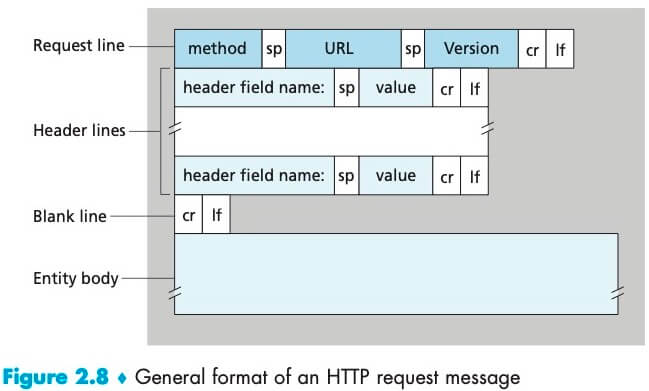
After the header lines (and the additional carriage return 回车 and line feed 换行) there is an “entity body.” The entity body is empty with the GET method, but is used with the POST method. If the value of the method field is POST, then the entity body contains what the user entered into the form fields.

A request generated with a form does not necessarily use the POST method. Instead, HTML forms often use the GET method and include the inputted data (in the form fields) in the requested URL.

Response Message

HTTP/1.1 200 OK
Date: Tue, 18 Aug 2015 15:44:04 GMT
Server: Apache/2.2.3 (CentOS)
Last-Modified: Tue, 18 Aug 2015 15:11:03 GMT
Content-Length: 6821
ETag: "526c3-f22-a88a4c80"
Accept-Ranges: bytes
Keep-Alive: timeout=max=100
Connection: Keep-Alive
Content-Type: text/html; charset=ISO-8859-1
(data data data data data ...)

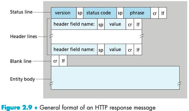
It has three sections: an initial status line, header lines, and then the entity body.

The status line has three fields: the protocol version field, a status code, and a corresponding status message.

常见的状态码包括：

Status code	说明
200 OK	请求成功
301 Moved Permanently	请求的对象被永久转移了，Client 将自动获取新 URL（位于响应报文的 Location: header line）
400 Bad Request	一个通用错误码，表示该请求不能被服务器理解
404 Not Found	被请求的文档不存在服务器上
505 HTTP Version Not Supported	服务器不支持请求报文使用的 HTTP 协议版本

For the header lines:

• The Date: header line indicates the time and date when the HTTP response was created and sent by the server.
• The Last-Modified: header line indicates the time and date when the object was created or last modified. It is critical for object caching, both in the local client and in proxy servers.
• The Content-Length: header line indicates the number of bytes in the object being sent.
• The Content-Type: header line indicates that the object in the entity body is HTML text. (The object type is officially indicated by the Content-Type: header and not by the file extension.)
• Either the client or the server can indicate to the other that it is going to close the persistent connection. It does so by including the header line Connection: close of the http request/reply.

HTTP 规范定义了许多的 header lines，header lines 可以被浏览器、服务器、代理服务器插入。这里提到的只是一小部分。

The entity body is the meat of the message—it contains the requested object itself (represented by data ...).

下面是响应报文的通用格式：

Cookie

We mentioned above that an HTTP server is stateless. This simplifies server design and has permitted engineers to develop high-performance Web servers that can handle thousands of simultaneous TCP connections. However, it is often desirable for a Web site to identify users, because it wants to serve content as a function of the user identity. For this purpose, HTTP uses cookies. Cookies allow sites to keep track of users.

Cookie technology has four components:

1. A cookie header line in the HTTP response message;
2. A cookie header line in the HTTP request message;
3. A cookie file kept on the user’s end system and managed by the user’s browser;
4. A back-end database at the Web site.

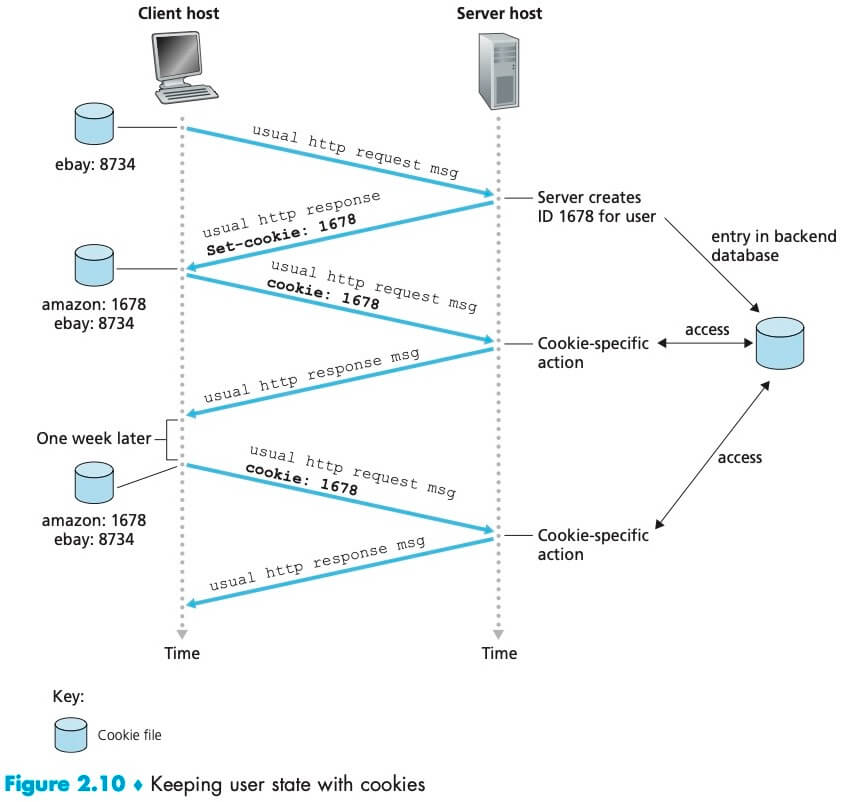
When Susan’s browser receives the HTTP response message, it sees the Set-cookie: header. The browser then appends a line to the special cookie file that it manages. This line includes the hostname of the server and the identification number in the Set-cookie: header.

We see that cookies can be used to identify a user. The first time a user visits a site, the user can provide a user identification. During the subsequent sessions, the browser passes a cookie header to the server, thereby identifying the user to the server. Cookies can thus be used to create a user session layer on top of stateless HTTP.

Web Caching and The Conditional GET

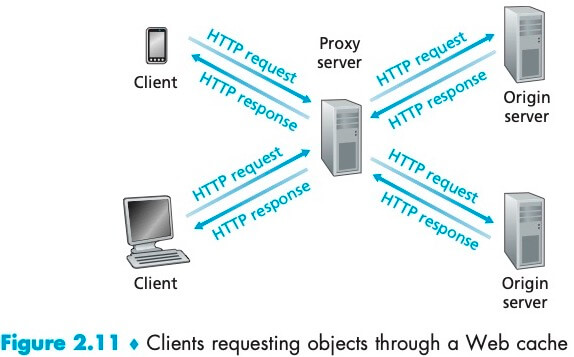
A Web cache—also called a proxy server—is a network entity that satisfies HTTP requests on the behalf of an origin Web server.

Web 缓存器有自己的磁盘存储空间，保存最近请求过的对象的副本。可以配置用户的浏览器，使得用户的所有 HTTP 请求首先指向 Web 缓存器。注意 Web cache 既是客户又是服务器。

Web 缓存器通常由 ISP 购买并安装。例如，一所大学可能在它的校园网安装 Web cache，并且将所有校园网上的用户浏览器配置为指向它。

在因特网上部署 Web cache 有两个原因。首先，Web cache 可以大大减少客户请求的响应时间；其次，Web 缓存器能够大大减少一个机构的接入链路到因特网的通信量，通过减少通信量，该机构就不必急于增加带宽，因此降低了费用。此外，Web 缓存器能从整体上大大减低因特网上的 Web 流量，从而改善了所有应用的性能。

通过使用内容分发网络 (Content Distribution Network, CDN)，Web cache 正在因特网中发挥着越来越重要的作用。CDN 公司在因特网上安装了许多地理上分散的缓存器，使大量流量实现了本地化。

Web cache 可以大大减少对客户请求的响应时间，但也引入了一个新的问题，即存放在 Web cache 中的对象副本可能是陈旧的。HTTP 协议有一种机制，允许 Web cache 证实它的对象是最新的，即 conditional GET。如果请求报文使用 GET 方法、并且请求报文中包含一个 If-Modified-Since: 的 header line，那么，这个 HTTP 请求报文就是一个条件 GET 请求报文。

HTTP/2

HTTP/2 [RFC 7540], standardized in 2015, was the first new version of HTTP since HTTP/1.1, which was standardized in 1997.

The primary goals for HTTP/2 are to reduce perceived latency by enabling request and response multiplexing over a single TCP connection, provide request prioritization and server push, and provide efficient compression of HTTP header fields.

HOL Blocking and HTTP/2 Framing

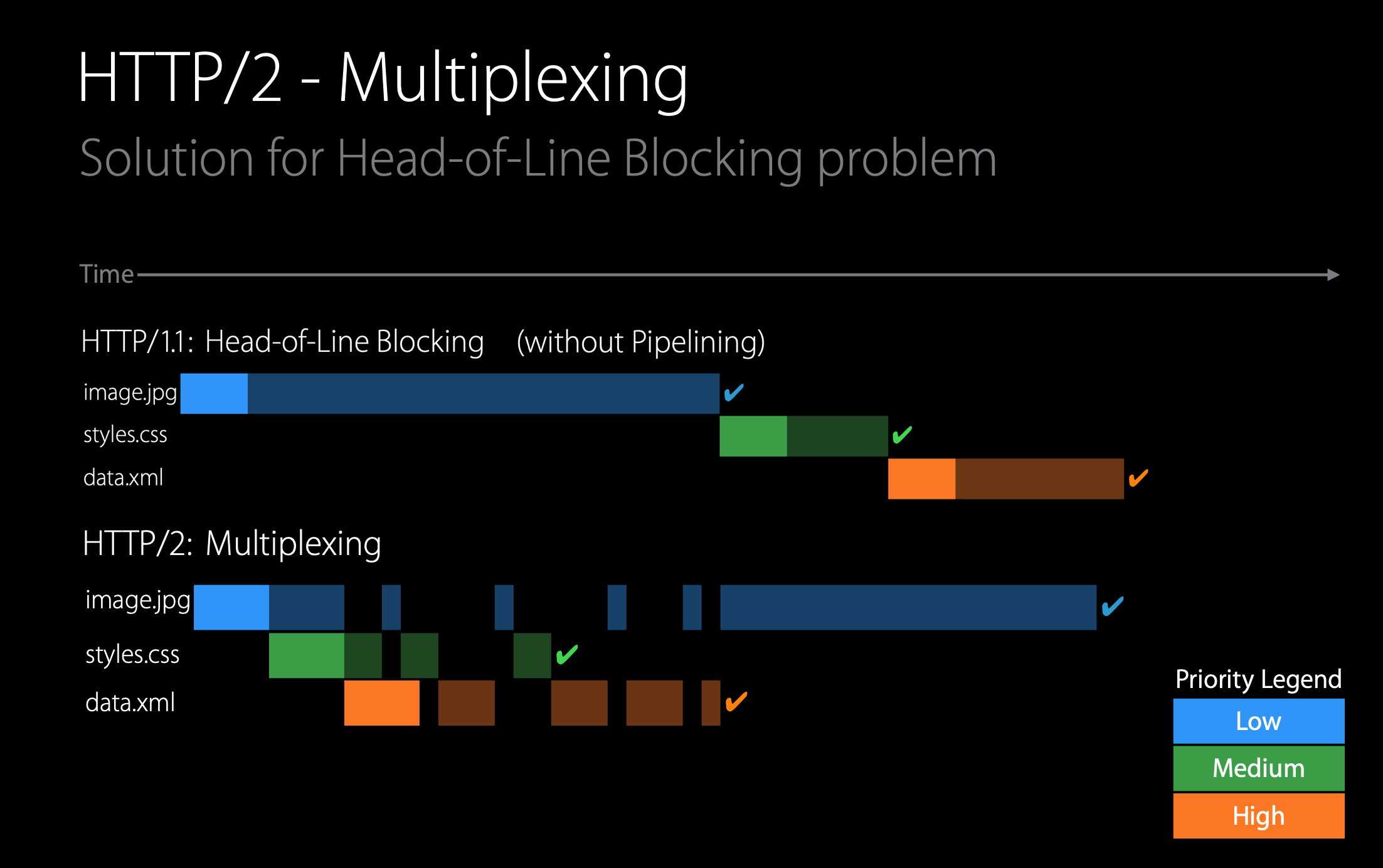
Developers of Web browsers discovered that sending all the objects in a Web page over a single TCP connection has a Head of Line (HOL) blocking problem. To understand HOL blocking, consider a Web page that includes an HTML base page, a large video clip near the top of Web page, and many small objects below the video. Using a single TCP connection, the video clip will take a long time to pass through the link, while the small objects are delayed as they wait behind the video clip; that is, the video clip at the head of the line blocks the small objects behind it.

HTTP/1.1 browsers typically work around this problem by opening multiple parallel TCP connections, thereby having objects in the same web page sent in parallel to the browser. This way, the small objects can arrive at and be rendered in the browser much faster, thereby reducing user-perceived delay.

TCP congestion control also provides browsers an unintended incentive 动机 to use multiple parallel TCP connections rather than a single persistent connection. Very roughly speaking, TCP congestion control aims to give each TCP connection sharing a bottleneck link an equal share of the available bandwidth of that link. By opening multiple parallel TCP connections to transport a single Web page, the browser can “cheat” and grab a larger portion of the link bandwidth. Many HTTP/1.1 browsers open up to six parallel TCP connections not only to circumvent HOL blocking but also to obtain more bandwidth.

One of the primary goals of HTTP/2 is to get rid of (or at least reduce the number of) parallel TCP connections for transporting a single Web page. This not only reduces the number of sockets that need to be open and maintained at servers, but also allows TCP congestion control to operate as intended.

The HTTP/2 solution for HOL blocking is to break each message into small frames, and interleave the request and response messages on the same TCP connection. The HTTP/2 framing mechanism can significantly decrease user-perceived delay.

WWDC 2015 - Networking with NSURLSession

The ability to break down an HTTP message into independent frames, interleave them, and then reassemble them on the other end is the single most important enhancement of HTTP/2. The framing is done by the framing sub-layer of the HTTP/2 protocol. When a server wants to send an HTTP response, the response is processed by the framing sub-layer, where it is broken down into frames. The header field of the response becomes one frame, and the body of the message is broken down into one for more additional frames. The frames of the response are then interleaved by the framing sub-layer in the server with the frames of other responses and sent over the single persistent TCP connection. As the frames arrive at the client, they are first reassembled into the original response messages at the framing sub-layer and then processed by the browser as usual. Similarly, a client’s HTTP requests are broken into frames and interleaved.

In addition to breaking down each HTTP message into independent frames, the framing sublayer also binary encodes the frames. Binary protocols are more efficient to parse, lead to slightly smaller frames, and are less error-prone.

How does HTTP/2 solve the Head of Line blocking (HOL) issue

HTTP/1.1 introduced a feature called "Pipelining" which allowed a client sending several HTTP requests back-to-back over the same TCP connection. However HTTP/1.1 still required the responses to arrive in order so it didn't really solved the HOL issue and as of today it is not widely adopted. In fact, it’s disabled on most popular desktop web browsers.

HTTP/2 solves the HOL issue by means of multiplexing requests over the same TCP connection, so a client can make multiple requests to a server without having to wait for the previous ones to complete as the responses can arrive in any order.

HTTP/2 does however still suffer from another type of HOL, as it runs over a TCP connection; and due to TCP's congestion control, one lost packet in a TCP stream makes all streams wait until that package is re-transmitted and received. This HOL is being addressed with the QUIC protocol.

Header compression (HPACK)

HPACK, a compression format for efficiently representing HTTP header fields, to be used in HTTP/2.

HPACK header compression is based on two tables, a static table and a dynamic table. The static table contains the most used HTTP headers and is unchangeable. The headers, which are not included in the static table, can be added to the dynamic table. The headers from the tables can be referenced by index.

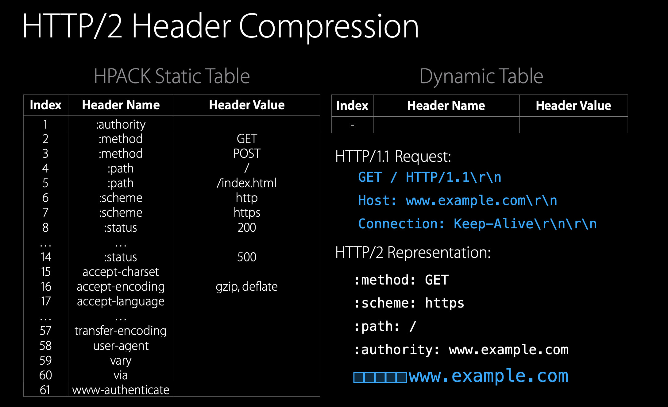
In this example, we need three bytes for the first three headers, plus an additional byte, which tells that we want to add the authority header to the dynamic table and the value of the authority with its length. And this is what is going to be sent to the server plus additional overhead for the header frame.

Now with the second request,（当我们再次请求时）HTTP/1.1 would send the same headers over and over again (textual protocol overhead). But you see that, in HTTP/2 case, the authority header goes in the dynamic table, we can reference all the headers using the static and the dynamic table. We are using only one byte for each header.

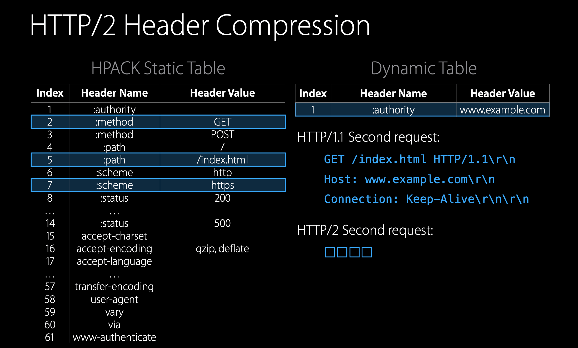
It is a huge savings of the bandwidth and it's remarkable how few bytes are needed to encode a request or response header in HTTP/2.

Response Message Prioritization

Message prioritization allows developers to customize the relative priority of requests to better optimize application performance. When a client sends concurrent requests to a server, it can prioritize the responses it is requesting by assigning a weight between 1 and 256 to each message. The higher number indicates higher priority. In addition to this, the client also states each message’s dependency on other messages by specifying the ID of the message on which it depends.

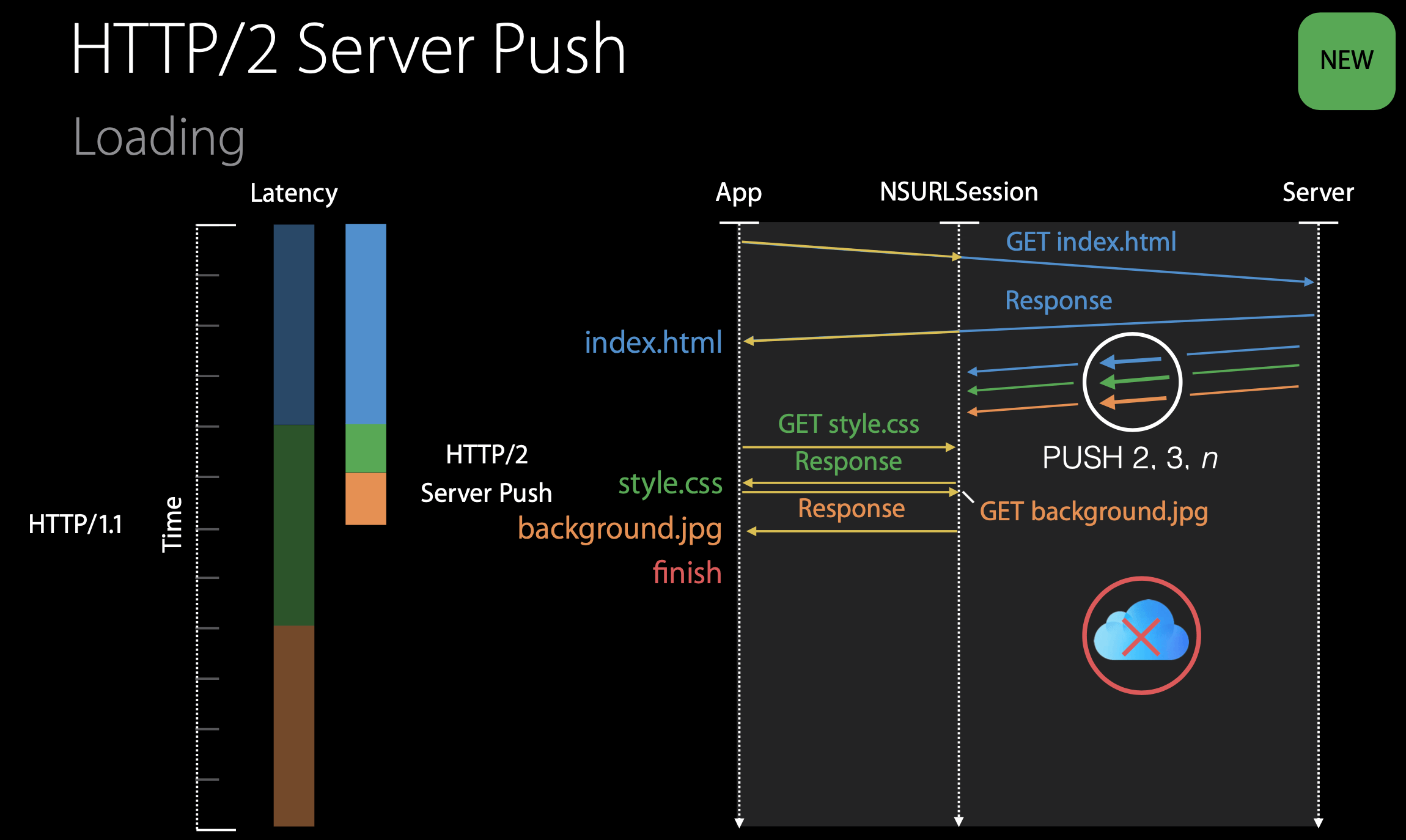
Server Pushing

Another feature of HTTP/2 is the ability for a server to send multiple responses for a single client request. That is, in addition to the response to the original request, the server can push additional objects to the client, without the client having to request each one. This is possible since the HTML base page indicates the objects that will be needed to fully render the Web page. So instead of waiting for the HTTP requests for these objects, the server can analyze the HTML page, identify the objects that are needed, and send them to the client before receiving explicit requests for these objects. Server push eliminates the extra latency due to waiting for the requests.

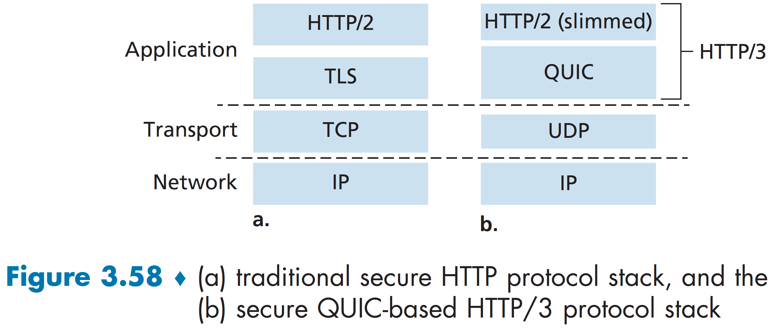
HTTP/3

Both HTTP/1.1 and HTTP/2 use TCP as their transport. QUIC, is a new protocol that is implemented in the application layer over the bare-bones UDP protocol. QUIC has several features that are desirable for HTTP, such as message multiplexing (interleaving), per-stream flow control, and low-latency connection establishment. QUIC is implemented over UDP where each stream is independent so that a lost packet only halts the particular stream to which the lost packet belongs, while the other streams can go on.

HTTP/3 is yet a new HTTP protocol that is designed to operate over QUIC. Many of the HTTP/2 features (such as message interleaving) are subsumed by QUIC, allowing for a simpler, streamlined design for HTTP/3.

HTTP/3 has TLS 1.3 security built right in and provides all the same multiplexed stream support as HTTP/2, but with further reductions to head-of-line blocking so that losses of any individual request or response won't hold up other potentially unrelated messages.

HTTP/3 also has higher fidelity information to provide improved congestion control and recovery of lost packets.

HTTP/3 also brings built-in mobility support such that network transitions don't cause in-progress operations to fail. They can instead seamlessly continue on the new network without interruption.

Email

Suppose Alice, with a Web-based e-mail account (such as Hotmail or Gmail), sends a message to Bob. The message is first sent from Alice’s browser to her mail server over HTTP(S). Alice’s mail server then sends the message to Bob’s mail server over SMTP. Bob then transfers the message from his mail server to his host over POP3.

DNS

一个 IP 地址由 4 个字节组成，例如 121.7.106.83，每个字节表示 0-255 的十进制数字。在因特网中，Host name 和 IP 地址都可以用来识别主机。人们在浏览器中习惯输入 host name，而路由器则喜欢定长的、有层次结构的 IP 地址。因此，我们需要有一种能进行主机名到 IP 地址转换的目录服务，这就是域名系统 (Domain Name System, DNS) 的主要任务。

DNS 有两层含义：1. 一个由分层的 DNS 服务器实现的分布式数据库；2. 一个使端系统能够查询分布式数据库的应用层协议。DNS 协议运行在 UDP 之上，使用 53 号端口。

DNS 请求为因特网应用带来了额外的时延，幸运的是，大部分 IP 地址通常就缓存在某个“附近的” DNS 服务器中。

除了主机名到 IP 地址的转换之外，DNS 还提供了以下服务：

• 主机别名 (host aliasing)。例如 relay1.west-coast.enterprise.com 称为规范主机名 (cannonical hostname)，它有两个别名 enterprise.com 和 www.enterprise.com。应用程序通过 DNS 服务来获得主机别名对应的规范主机名以及 IP 地址。
• 邮件服务器别名 (mail server aliasing)。
• 负载分配 (load distribution)。繁忙的站点如 cnn.com 被分布在多台服务器上，每个都拥有不同的 IP 地址，多个 IP 地址可以映射到同一个规范主机名。DNS 在所有这些服务器之间进行负载分配。

DNS 是一个在因特网上实现分布式数据库的精彩范例。大量的 DNS 服务器以层次方式组织、分布在全世界范围内。大致上，有 3 种类型的 DNS 服务器。

• Root DNS servers. There are over 400 root name servers scattered all over the world. Root name servers provide the IP addresses of the TLD servers.
• Top-level domain (TLD) servers. For each of the top-level domains such as com, org, net, edu, and gov, and all of the country top-level domains such as uk, fr, ca, and jp — there is TLD server (or server cluster). TLD servers provide the IP addresses for authoritative DNS servers.
• Authoritative DNS servers. Every organization with publicly accessible hosts on the Internet must provide publicly accessible DNS records. An organization can choose to implement its own authoritative DNS server to hold these records; alternatively, the organization can pay to have these records stored in an authoritative DNS server of some service provider.

The root, TLD, and authoritative DNS servers all belong to the hierarchy of DNS servers. There is another important type of DNS server called the local DNS server. Each ISP—such as a residential ISP or an institutional ISP—has a local DNS server.

When a host connects to an ISP, the ISP provides the host with the IP addresses of one or more of its local DNS servers (typically through DHCP). When a host makes a DNS query, the query is sent to the local DNS server, which acts a proxy, forwarding the query into the DNS server hierarchy.

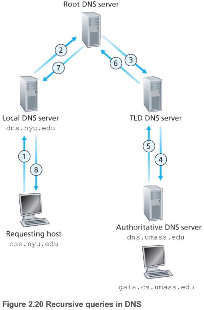
如下图所示，Client 想要访问主机 gaia.cs.umass.edu：

1. Client sends a DNS query message to its local DNS server.
2. The local DNS server forwards the query message to a root DNS server.
3. The root DNS server takes note of the edu suffix and returns a list of IP addresses for TLD servers responsible for edu.
4. The local DNS server then resends the query message to one of these TLD servers.
5. The TLD server takes note of the umass.edu suffix and responds with the IP address of the authoritative DNS server for the University of Massachusetts, namely, dns.umass.edu.
6. Finally, the local DNS server resends the query message directly to dns.umass.edu.
7. Authoritative DNS server responds with the IP address of gaia.cs.umass.edu.
8. Local DNS server responds with the IP address of gaia.cs.umass.edu to client.

实际上，为了改善时延、减少因特网上到处传输的 DNS 报文数量，DNS 广泛使用了缓存技术。缓存原理十分简单，在一个请求链中，当某 DNS 服务器接收一个响应后，它能将映射缓存在服务器本地存储中。当新的、对相同主机名的查询到达时，就能直接提供 IP 地址。由于主机名和 IP 地址之间的映射不是永久的，DNS 服务器在一段时间后将丢弃缓存的信息。

DNS 服务器上存储了资源记录 (Resource Record, RR)。RR 提供了主机名到 IP 地址的映射。每个 DNS 响应报文包含一条或多条 RR。

RR 是一个包含了下列字段的四元组：(Name, Value, Type, TLL)。TLL 是该记录的生存时间，它决定了 RR 应当从缓存中删除的时间。

• If Type=A, then Name is a hostname and Value is the IP address for the hostname. As an example, (relay1.bar.foo.com, 145.37.93.126, A) is a Type A record.
• If Type=NS, then Name is a domain (such as foo.com) and Value is the hostname of an authoritative DNS server that knows how to obtain the IP addresses for hosts in the domain. As an example, (foo.com, dns.foo.com, NS) is a Type NS record.
• If Type=CNAME, then Value is a canonical hostname for the alias hostname Name. As an example, (foo.com, relay1.bar.foo.com, CNAME) is a CNAME record.
• If Type=MX, then Value is the canonical name of a mail server that has an alias hostname Name.

查看当前 DNS：nslookup domain

查询域名对应的 IP：nslookup www.baidu.com

查询 A 记录：nslookup -query=A www.baidu.com

查询 CNAME 记录：nslookup -query=CNAME www.baidu.com

P2P

考虑从因特网上下载一个文件。在客户-服务器文件分发中，该服务器必须向每个 peer 发送该文件的一个副本；在 P2P 文件分发中，每个 peer 能够向其他 peers 分发它已经收到的该文件的部分，从而在分发过程中协助该服务器。到 2016 年止，最为流行的 P2P 文件分发协议是 BitTorrent。

用 BitTorrent 的术语来讲，参与一个特定文件分发的所有 peers 的集合被称为一个洪流 (torrent)。在一个洪流中的 peers 彼此下载等长度的文件块 (chunk)，典型的块长度为 256KB。当一个 peer 首次加入一个洪流时，它没有块。随着时间的流逝，它累积了越来越多的块。当它下载块时，也为其他 peers 上载了多个块。一旦某个 peer 获得了整个文件，它也许（自私地）离开洪流，或继续留在该洪流中并继续向其他 peers 上载块。同时，任何 peer 可能在任何时候仅具有块的子集就离开该洪流，并在以后重新加入该洪流中。

每个洪流具有一个基础设施节点，称为追踪器 (tracker)。当一个 peer 加入某洪流时，它向追踪器注册自己，并周期性地通知追踪器它仍在该洪流中。以这种方式，追踪器跟踪参与在洪流中的 peers。一个给定的洪流可能在任何时刻具有数以百计或数以千计的 peers。

当一个新的 peer，Alice 加入该洪流时，追踪器随机地从参与该洪流的 peers 集合中选择一个子集（假设选择了 50 个 peers），并将它们的 IP 地址发送给 Alice。Alice 则试图与这 50 个 peers 创建并行的 TCP 连接。随着时间的流逝，这些 peers 中的某些可能离开，其他 peers（最初 50 个以外的）也可能与 Alice 创建 TCP 连接。因此一个 peer 的 neighboring peers 将随时间而波动。

在任意时刻，每个 peer 可能具有该文件的块的子集，不同的 peers 可能具有不同的子集。Alice 周期性地经 TCP 连接询问每个 neighboring peer 它们所具有的块列表。如果 Alice 具有 L 个不同的邻居，她将获得 L 个块列表。有了这个信息，Alice 将做出两个重要决定。第一，她应当向邻居请求哪些块呢？第二，她应当向哪些向她请求块的邻居发送块呢？

在决定请求哪些块的过程中，BitTorrent 使用一种称为最稀缺优先 (rarest first) 的技术。最稀缺的块，就是那些在她的邻居中副本数量最少的块)，Alice 首先请求那些最稀缺的块。这样，最稀缺的块将得到更为迅速的重新分发，这样做的目的是大致地均衡每个块在洪流中的副本数量。

为了决定她响应哪个请求，BitTorrent 使用了一种聪明的交易算法。其基本想法是，Alice 给予当前向她提供数据的邻居中速率最高的那些以优先权。Alice 对于她的每个邻居都持续地测量接收速率，并确定流入速率最高的 4 个邻居。每过 10 秒，她重新计算该速率并可能修改这 4 个 peers 的集合，我们称这 4 个 peers 被 unchoked。重要的是，每过 30 秒，她也要随机地选择另外一个邻居（不在这 4 个 peers 里）Bob 并向其发送块。因为 Alice 正在向 Bob 发送数据，她可能成为 Bob 前 4 位上载者之一，这样的话 Bob 将开始向 Alice 发送数据。如果 Bob 向 Alice 发送数据的速率足够高，Bob 接下来也能成为 Alice 的前 4 位上载者。这种设计的效果是 peers 能够在洪流中，始终趋向于找到那些以最快速率交换文件块的邻居。对于 Alice，除了这 4 个 peers 和一个每隔一段时间就随机选择的试探性 peer，其它所有 neighboring peers 都被 choked，即它们不会从 Alice 这里接收到任何块。

BitTorrent 还有一些有趣的机制没有在这里讨论。但总体来说，BitTorrent 取得了广泛成功，它的设计使得无数个 peers 在无数个洪流中积极地共享文件。

Video Streaming

From a networking perspective, perhaps the most salient characteristic of video is its high bit rate. For example, a single 2 Mbps video with a duration of 67 minutes will consume 1 gigabyte of storage and traffic. By far, the most important performance measure for streaming video is average end-to-end throughput. In order to provide continuous playout, the network must provide an average throughput to the streaming application that is at least as large as the bit rate of the compressed video. We can also use compression to create multiple versions of the same video, each at a different quality level.

In HTTP streaming, the video is simply stored at an HTTP server as an ordinary file with a specific URL. On the client side, the bytes are collected in a client application buffer. The streaming video application periodically grabs video frames from the client application buffer, decompresses the frames, and displays them on the user’s screen.

Although HTTP streaming has been extensively deployed in practice, it has a major shortcoming: All clients receive the same encoding of the video, despite the large variations in the amount of bandwidth available to a client. This has led to the development of a new type of HTTP-based streaming, often referred to as Dynamic Adaptive Streaming over HTTP (DASH).

In DASH, the video is encoded into several different versions, with each version having a different bit rate. Each video version is stored in the HTTP server, each with a different URL. The HTTP server also has a manifest file, which provides a URL for each version along with its bit rate. The client first requests the manifest file and learns about the various versions. The client then selects one chunk at a time by specifying a URL and a byte-range in an HTTP GET request message header for each chunk. While downloading chunks, the client also measures the received bandwidth and runs a rate determination algorithm to select the chunk to request next. Naturally, if the client has a lot of video buffered and if the measured receive bandwidth is high, it will choose a chunk from a high-bitrate version. And naturally if the client has little video buffered and the measured received bandwidth is low, it will choose a chunk from a low-bitrate version. DASH therefore allows the client to freely switch among different quality levels.

Content Distribution Networks

为了应对向分布于全世界的用户分发巨量视频数据的挑战，视频流公司都会利用内容分发网络 (Content Distribution Network, CDN)。一个 CDN 管理着分布在多个地理位置上的服务器，这些服务器上存储着视频等资源文件的副本，并且总是将每个用户请求定向到最优的 CDN 位置。CDN 可以是专用 CDN (privace CDN)，它由内容提供商私人所有；也可以是第三方 CDN (third-party CDN)，它代表多个内容提供商分发内容。

CDN 的服务器是如何部署的呢？CDNs typically adopt one of two different server placement philosophies: Enter Deep (deploying server clusters in access ISPs); Bring Home (place their clusters in IXPs).

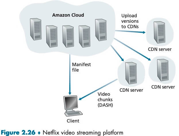
一旦 CDN 的集群准备就绪，它就可以跨集群复制内容。CDN 不会将每个视频的副本放置在每个集群中，因为某些视频很少观看或仅在某些国家中流行。而是使用一种简单的拉策略：如果客户向一个未存储该视频的集群请求某视频，则该集群检索该视频（从某中心仓库或者从另一个集群），向客户流式传输视频时的同时、在本地存储一个副本。当某集群存储器变满时，它删除不经常请求的视频。除了拉策略，当然还有其它策略，Netflix CDN 使用 push caching 而不是 pull caching：内容在非高峰时段被推入服务器，而不是在缓存未命中时拉取。

当客户端检索某个资源时，CDN 必须截获该请求，以便能够——1. 确定此时适合用于该客户的 CDN 服务器集群；2. 将客户的请求重定向到该集群的某台服务器。大多数 CDN 利用 DNS 来截获和重定向请求。

Socket Programming

Processes residing in two different end systems communicate with each other by reading from, and writing to, sockets.

网络应用程序有两类。一类是由协议标准（如一个 RFC）中所定义的操作的实现，客户端和服务端必须遵守该 RFC 的规则；另一类是专用的应用程序，其应用层协议没有公开发布在某 RFC 中或其他地方，不知道这个协议的开发者无法开发出能与之通信的应用程序。

UDP

When a socket is created, an identifier, called a port number, is assigned to it. The sending process attaches to the packet a destination address, which consists of the destination host’s IP address and the destination socket’s port number.

client.py

from socket import *

serverName = '127.0.0.1'
serverPort = 12000
clientSocket = socket(AF_INET, SOCK_DGRAM) # 1

message = input('Input lowercase sentence:')
clientSocket.sendto(message.encode(), (serverName, serverPort)) # 2,3

modifiedMessage, serverAddress = clientSocket.recvfrom(2048) # 4
print(modifiedMessage.decode())
clientSocket.close()

[1] The first parameter indicates the address family; in particular, AF_INET indicates that the underlying network is using IPv4. The second parameter indicates that the socket is of type SOCK_DGRAM, which means it is a UDP socket (rather than a TCP socket).

[2] Note that we are not specifying the port number of the client socket when we create it; we are instead letting the operating system do this for us.

[3] encode convert the message from string type to byte type.

[4] The maximum amount of data to be received is specified as 2048 bytes in the buffer size.

server.py

from socket import *

serverPort = 12000
serverSocket = socket(AF_INET, SOCK_DGRAM)
serverSocket.bind(('', serverPort)) # 1
print('The server is ready to receive')

while True:
    message, clientAddress = serverSocket.recvfrom(2048)
    modifiedMessage = message.decode().upper()
    serverSocket.sendto(modifiedMessage.encode(), clientAddress)

[1] bind binds (that is, assigns) the port number 12000 to the server’s socket. In this manner, when anyone sends a packet to port 12000 at the server, that packet will be directed to this socket.

TCP

Unlike UDP, TCP is a connection-oriented protocol. This means that before the client and server can start to send data to each other, they first need to handshake and establish a TCP connection. After that, they just drop the data into the TCP connection via sockets. This is different from UDP, for which the server must attach a destination address to the packet before dropping it into the socket.

What is meant by a handshaking protocol? A protocol uses handshaking if the two communicating entities first exchange control packets before sending data to each other. SMTP uses handshaking at the application layer whereas HTTP does not.

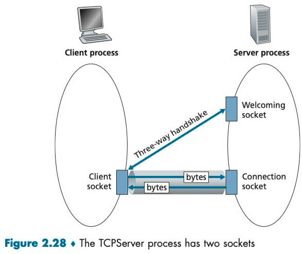
With the server process running, the client process can initiate a TCP connection to the server. This is done in the client program by creating a TCP socket. When the client creates its TCP socket, it specifies the address of the welcoming socket in the server, namely, the IP address of the server host and the port number of the socket.

During the three-way handshake, when the server “hears” the knocking, it creates a new connection socket that is dedicated to that particular client.

client.py

from socket import *

serverName = '127.0.0.1'
serverPort = 12000
clientSocket = socket(AF_INET, SOCK_STREAM)
clientSocket.connect((serverName, serverPort))

sentence = input('Input lowercase sentence:')
clientSocket.send(sentence.encode()) # 1

modifiedSetence = clientSocket.recv(1024)
print('From Server:', modifiedSetence.decode())

clientSocket.close()

[1] This line sends the sentence through the client’s socket and into the TCP connection. Note that the program does not explicitly create a packet and attach the destination address to the packet, as was the case with UDP sockets.

from socket import *
serverPort = 12000
serverSocket = socket(AF_INET, SOCK_STREAM)
serverSocket.bind(('', serverPort))
serverSocket.listen(1) ## the maximum number of queued connections (at least 1)
print('The server is ready to receive')
while True:
    connectionSocket, addr = serverSocket.accept()
    sentence = connectionSocket.recv(1024).decode()
    capitalizedSentence = setence.upper()
    connectionSocket.send(capitalizedSentence.encode())
    connectionSocket.close()
serverSocket.close()

When a client knocks on this door, the program invokes the accept() method for serverSocket, which creates a new socket in the server, called connectionSocket, dedicated to this particular client.

With the UDP server, there is no welcoming socket, and all data from different clients enters the server through one single socket. With the TCP server, there is a welcoming socket, thus, to support n simultaneous connections, the server would need n+1 sockets.

Exercise: Proxy Server

Write a simple TCP program for a server that accepts lines of input from a client and prints the lines onto the server’s standard output.

from socket import *
serverPort = 12000
serverSocket = socket(AF_INET, SOCK_STREAM)
serverSocket.bind(('', serverPort))
serverSocket.listen(1)
while True:
    connectionSocket, addr = serverSocket.accept()
    sentence = connectionSocket.recv(1024).decode()
    print(sentence)
    connectionSocket.send("Hello world!".encode())
    connectionSocket.close()
serverSocket.close()

On the Web browser, set the proxy server to your running server program. Your browser should now send its GET request messages to your server, and your server should display the messages on its standard output.

CONNECT www.baidu.com:443 HTTP/1.1
Host: www.baidu.com:443
Proxy-Connection: keep-alive
User-Agent: Mozilla/5.0 (Macintosh; Intel Mac OS X 11_2_3) AppleWebKit/537.36 (KHTML, like Gecko) Chrome/89.0.4389.90 Safari/537.36
......

Transport Layer

Transport-layer protocols are implemented in the end systems but not in network routers. On the sending side, the transport layer converts the application-layer messages into segments. This is done by (possibly) breaking the application messages into smaller chunks and adding a transport-layer header to each chunk to create the transport-layer segment. The transport layer then passes the segment to the network layer at the sending end system, where the segment is encapsulated within a network-layer packet (a datagram) and sent to the destination. It’s important to note that network routers act only on the network-layer fields of the datagram; that is, they do not examine the fields of the transport-layer segment encapsulated with the datagram. On the receiving side, the network layer extracts the transport-layer segment from the datagram and passes the segment up to the transport layer. The transport layer then processes the received segment, making the data in the segment available to the receiving application.

Before proceeding with our introduction of UDP (User Datagram Protocol) and TCP (Transmission Control Protocol), it will be useful to say a few words about the Internet’s network layer. IP, for Internet Protocol, is a best-effort delivery service. This means that IP makes its “best effort” to deliver segments between communicating hosts, but it makes no guarantees.

Extending host-to-host delivery to process-to-process delivery is called transport-layer multiplexing and demultiplexing.（多路复用、多路分解）UDP and TCP also provide integrity checking by including error-detection fields in their segments’ headers. These two minimal transport-layer services are the only two that UDP provides!

TCP, on the other hand, offers several additional services to applications.

• First and foremost, it provides reliable data transfer. Using flow control, sequence numbers, acknowledgments, and timers, TCP ensures that data is delivered from sending process to receiving process, correctly and in order.
• TCP also provides congestion control. Congestion control is not so much a service provided to the invoking application as it is a service for the Internet as a whole.

Multiplexing and Demultiplexing

This job of delivering the data in a transport-layer segment to the correct socket is called demultiplexing. The job of gathering data chunks at the source host from different sockets, encapsulating each data chunk with header information (that will later be used in demultiplexing) to create segments, and passing the segments to the network layer is called multiplexing.

There are source port number field and the destination port number field in a transport-layer segment. Each port number is a 16-bit number, ranging from 0 to 65535. The port numbers ranging from 0 to 1023 are called well-known port numbers and are restricted, which means reserved for use by well-known application protocols such as HTTP.

Each socket in the host could be assigned a port number, and when a segment arrives at the host, the transport layer examines the destination port number in the segment and directs the segment to the corresponding socket. The segment’s data then passes through the socket into the attached process. As we’ll see, this is basically how UDP does it.

It is important to note that a UDP socket is fully identified by a two-tuple consisting of a destination IP address and a destination port number. As a consequence, if two UDP segments have different source IP addresses and/or source port numbers, but have the same destination IP address and destination port number, then the two segments will be directed to the same destination process via the same destination socket. In UDP, the source port number serves as part of a “return address”.

TCP socket is identified by a four-tuple: (source IP address, source port number, destination IP address, destination port number). In particular, and in contrast with UDP, two arriving TCP segments with different source IP addresses or source port numbers will (with the exception of a TCP segment carrying the original connection-establishment request) be directed to two different sockets.

Today’s high-performing Web servers often use only one process, and create a new thread with a new connection socket for each new client connection. For such a server, at any given time there may be many connection sockets (with different identifiers) attached to the same process. If the client and server are using persistent HTTP, then throughout the duration of the persistent connection the client and server exchange HTTP messages via the same server socket.

UDP

Note that with UDP there is no handshaking between sending and receiving transport-layer entities before sending a segment. For this reason, UDP is said to be connectionless.

DNS is an example of an application-layer protocol that typically uses UDP. The DNS application at the querying host then waits for a reply to its query. If it doesn’t receive a reply (possibly because the underlying network lost the query or the reply), it might try resending the query, try sending the query to another name server, or inform the invoking application that it can’t get a reply.

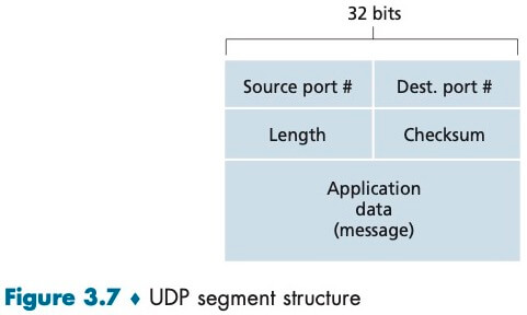
The UDP header has only four fields, each consisting of two bytes, totally 8 bytes. The length field specifies the number of bytes in the UDP segment (header plus data). The checksum is used by the receiving host to check whether errors have been introduced into the segment. In truth, the checksum is also calculated over a few of the fields in the IP header in addition to the UDP segment.

Although UDP provides error checking, it does not do anything to recover from an error. Some implementations of UDP simply discard the damaged segment; others pass the damaged segment to the application with a warning.

Some applications are better suited for UDP (rather than TCP) for the following reasons:

• Finer application-level control over what data is sent, and when.
  • WHAT: With TCP, the application writes data to the connection send buffer and TCP will grab bytes without necessarily putting a single message in the TCP segment; TCP may put more or less than a single message in a segment. UDP, on the other hand, encapsulates in a segment whatever the application gives it; so that, if the application gives UDP an application message, this message will be the payload of the UDP segment. Thus, with UDP, an application has more control of what data is sent in a segment.
  • WHEN: With TCP, due to flow control and congestion control, there may be significant delay from the time when an application writes data to its send buffer until when the data is given to the network layer. UDP does not have delays due to flow control and congestion control.
• No connection establishment. UDP does not introduce any delay to establish a connection. The TCP connection-establishment delay in HTTP is an important contributor to the delays associated with downloading Web documents.
• No connection state. A server devoted to a particular application can typically support many more active clients when the application runs over UDP rather than TCP.
• Small packet header overhead. The TCP segment has 20 bytes of header over- head in every segment, whereas UDP has only 8 bytes of overhead.

TCP

Go-Back-N (GBN) and Selective Repeat (SR)

In a Go-Back-N (GBN) protocol, the sender is allowed to transmit multiple packets (when available) without waiting for an acknowledgment, but is constrained to have no more than some maximum allowable number, N, of unacknowledged packets in the pipeline.

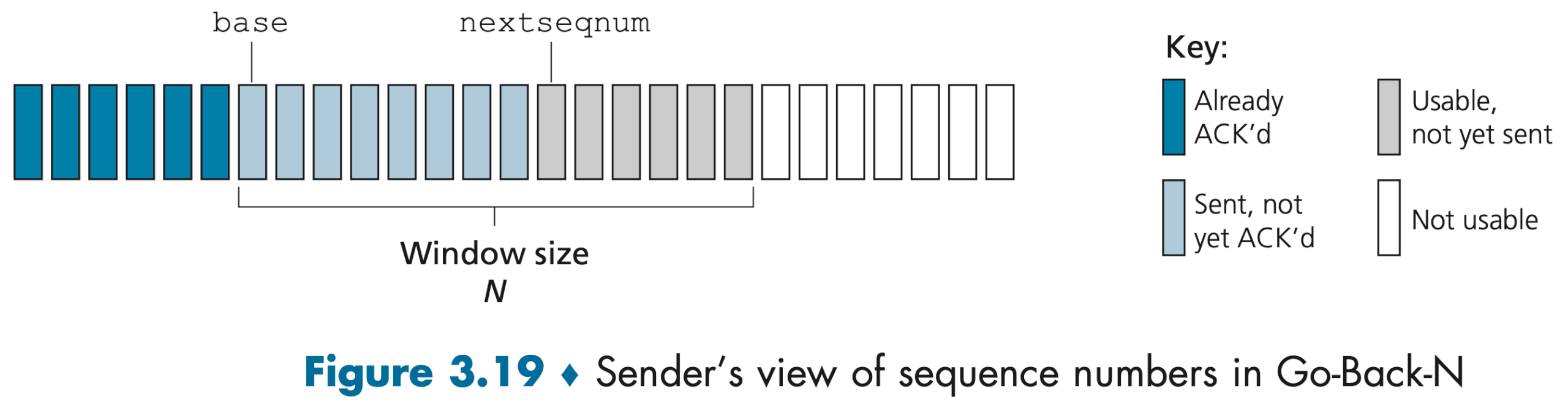
Four intervals in the range of sequence numbers can be identified:

• packets that have already been transmitted and acknowledged
• packets that have been sent but not yet acknowledged
• can be used for packets that can be sent immediately
• cannot be used until an unacknowledged packet currently in the pipeline has been acknowledged

As the protocol operates, this window slides forward over the sequence number space. For this reason, N is often referred to as the window size and the GBN protocol itself as a sliding-window protocol. N is limited by flow control and congestion control.

When rdt_send() is called from above, the sender first checks to see if the window is full, that is, whether there are N outstanding, unacknowledged packets. If the window is not full, a packet is created and sent, and variables are appropriately updated. If the window is full, the sender simply returns the data back to the upper layer, an implicit indication that the window is full. The upper layer would presumably then have to try again later. In a real implementation, the sender would more likely have either buffered (but not immediately sent) this data, or would have a synchronization mechanism (for example, a semaphore or a flag) that would allow the upper layer to call rdt_send() only when the window is not full.

Selective-repeat protocols avoid unnecessary retransmissions by having the sender retransmit only those packets that it suspects were received in error (that is, were lost or corrupted) at the receiver. This individual, as-needed, retransmission will require that the receiver individually acknowledge correctly received packets. A window size of N will again be used to limit the number of outstanding, unacknowledged packets in the pipeline. However, unlike GBN, the sender will have already received ACKs for some of the packets in the window.

TCP Connection

TCP is said to be connection-oriented because before one application process can begin to send data to another, the two processes must first “handshake” with each other. Both sides of the connection will initialize many TCP state variables.

Recall that because the TCP protocol runs only in the end systems and not in the intermediate network elements (routers and link-layer switches), the intermediate network elements do not maintain TCP connection state.

A TCP connection provides a full-duplex service: The application-layer data can flow from Process A to Process B at the same time as application-layer data flows from Process B to Process A.

Suppose a process running in one host wants to initiate a connection with another process in another host. Recall that the process that is initiating the connection is called the client process, while the other process is called the server process. Because three segments are sent between the two hosts, this connection-establishment procedure is often referred to as a three-way handshake.

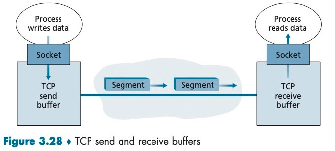
Once a TCP connection is established, the two application processes can send data to each other. Let’s consider the sending of data from the client process to the server process. The client process passes a stream of data through the socket. Once the data passes through the door, the data is in the hands of TCP running in the client. TCP directs this data to the connection’s send buffer, which is one of the buffers that is set aside during the initial three-way handshake. From time to time, TCP will grab chunks of data from the send buffer and pass the data to the network layer. Interestingly, the TCP specification [RFC 793] is very laid back about specifying when TCP should actually send buffered data, stating that TCP should “send that data in segments at its own convenience.”

The maximum amount of data that can be grabbed and placed in a segment is limited by the maximum segment size (MSS). The MSS is typically set by first determining the length of the largest link-layer frame that can be sent by the local sending host (the so-called maximum transmission unit, MTU), and then setting the MSS to ensure that a TCP segment (when encapsulated in an IP datagram) plus the TCP/IP header length (typically 40 bytes) will fit into a single link-layer frame. Both Ethernet and PPP link-layer protocols have an MTU of 1,500 bytes. Thus, a typical value of MSS is 1460 bytes. Note that the MSS is the maximum amount of application-layer data in the segment, not the maximum size of the TCP segment including headers.

TCP pairs each chunk of client data with a TCP header, thereby forming TCP segments. The segments are passed down to the network layer, where they are separately encapsulated within network-layer IP datagrams. The IP datagrams are then sent into the network. When TCP receives a segment at the other end, the segment’s data is placed in the TCP connection’s receive buffer. Each side of the connection has its own send buffer and its own receive buffer.

TCP Segment

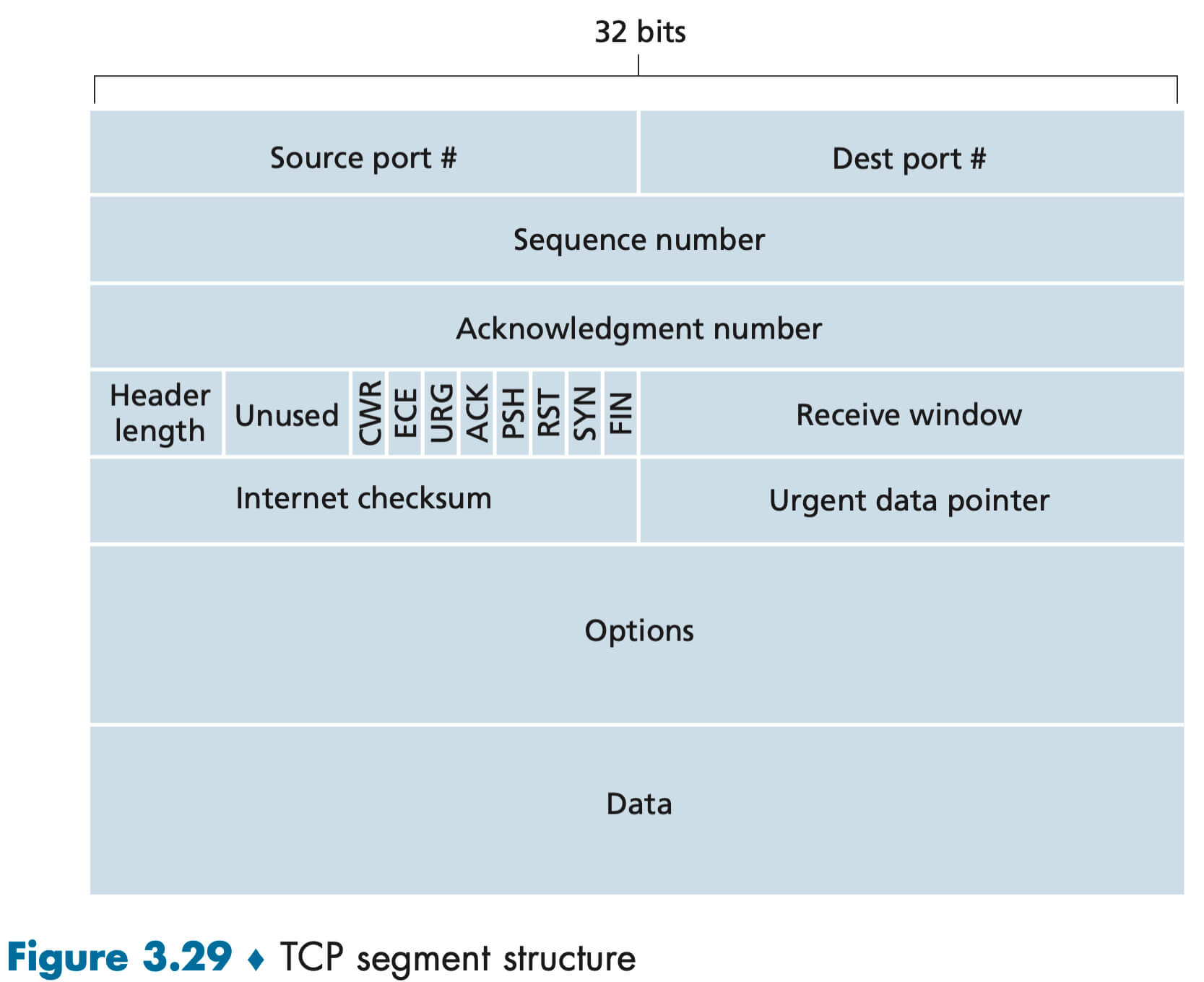
The TCP segment consists of header fields and a data field. TCP header is typically 20 bytes. The data field contains a chunk of application data.

As with UDP, the header includes source and destination port numbers, which are used for multiplexing/ demultiplexing data from/to upper-layer applications. Also, as with UDP, the header includes a checksum field. A TCP segment header also contains the following fields:

• The 32-bit sequence number field and the 32-bit acknowledgment number field are used by the TCP sender and receiver in implementing a reliable data transfer service.
• The 16-bit receive window field is used for flow control.
• The 4-bit header length field specifies the length of the TCP header (typically 20 bytes).
• The ACK bit is used to indicate that the segment contains an acknowledgment for a segment that has been successfully received.
• The RST, SYN, and FIN bits are used for connection setup and teardown.
• The CWR and ECE bits are used in explicit congestion notification.

TCP views data as an unstructured, but ordered, stream of bytes. The sequence number for a segment is therefore the byte-stream number of the first byte in the segment.

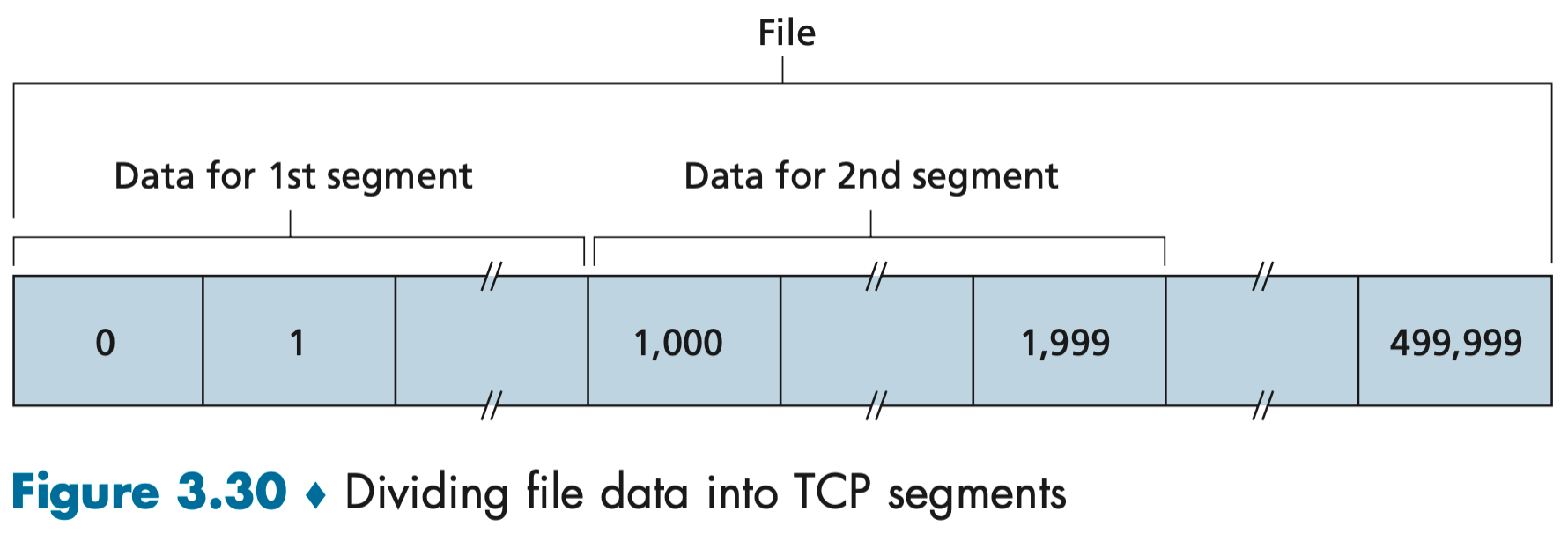
Suppose that a process in Host A wants to send a stream of data to a process in Host B over a TCP connection. The TCP in Host A will implicitly number each byte in the data stream. Suppose that the data stream consists of a file consisting of 500,000 bytes, that the MSS is 1,000 bytes, and that the first byte of the data stream is numbered 0. As shown in Figure 3.30, TCP constructs 500 segments out of the data stream. The first segment gets assigned sequence number 0, the second segment gets assigned sequence number 1,000, the third segment gets assigned sequence number 2,000, and so on. Each sequence number is inserted in the sequence number field in the header of the appropriate TCP segment.

Recall that TCP is full-duplex, the acknowledgment number that Host A puts in its segment is the sequence number of the next byte Host A is expecting from Host B.

Suppose that Host A has received one segment from Host B containing bytes 0 through 535 and another segment containing bytes 900 through 1,000. For some reason Host A has not yet received bytes 536 through 899. In this example, Host A is still waiting for byte 536 (and beyond) in order to re-create B’s data stream. Thus, A’s next segment to B will contain 536 in the acknowledgment number field. Because TCP only acknowledges bytes up to the first missing byte in the stream, TCP is said to provide cumulative acknowledgments 累积确认. The receiver keeps the out-of-order bytes and waits for the missing bytes to fill in the gaps.

在图 3-30 中，我们假设初始序号为 0。实际上，TCP 连接的双方随机地选择初始序号。这样做可以减少将那些仍在网络中存在的、来自两台主机之间先前已终止的连接的报文段，误认为是后来这两台主机之间新建连接所产生的有效报文段的可能性（它碰巧与旧连接使用了相同的端口号）。

Round-Trip Time Estimation and Timeout

TCP uses a timeout/retransmit mechanism to recover from lost segments. Perhaps the most obvious question is the length of the timeout intervals. Clearly, the timeout should be larger than the connection’s round-trip time (RTT). Otherwise, unnecessary retransmissions would be sent.

How TCP estimates the round-trip time between sender and receiver? The sample RTT, denoted SampleRTT, for a segment is the amount of time between when the segment is sent (that is, passed to IP) and when an acknowledgment for the segment is received. At any point in time, the SampleRTT is being estimated for only one of the transmitted but currently unacknowledged segments, leading to a new value of SampleRTT approximately once every RTT. Also, TCP never computes a SampleRTT for a segment that has been retransmitted; it only measures SampleRTT for segments that have been transmitted once.

Obviously, the SampleRTT values will fluctuate. Upon obtaining a new SampleRTT, TCP updates EstimatedRTT according to the following formula:

EstimatedRTT = (1 – α) * EstimatedRTT + α * SampleRTT (The recommended value of α is 0.125)

Note that EstimatedRTT is a weighted average of the SampleRTT values.

It is also valuable to have a measure of the variability of the RTT: DevRTT, an estimate of how much SampleRTT typically deviates from EstimatedRTT.

DevRTT = (1 – β) * DevRTT + β * |SampleRTT – EstimatedRTT| (The recommended value of β is 0.25)

It is therefore desirable to set the timeout equal to the EstimatedRTT plus some margin:

TimeoutInterval = EstimatedRTT + 4 * DevRTT

An initial TimeoutInterval value of 1 second is recommended [RFC 6298]. Also, when a timeout occurs, the value of TimeoutInterval is doubled to avoid a premature timeout occurring for a subsequent segment that will soon be acknowledged. However, as soon as a segment is received and EstimatedRTT is updated, the TimeoutInterval is again computed using the formula above.

Reliable Data Transfer

We should keep in mind that reliable data transfer can be provided by link-, network-, transport-, or application-layer protocols.

The TCP timer management procedures use only a single retransmission timer, even if there are multiple transmitted but not yet acknowledged segments. It is helpful to think of the timer as being associated with the oldest unacknowledged segment.

Whenever the timeout event occurs, TCP retransmits the not-yet-acknowledged segment with the smallest sequence number, sets the next timeout interval to twice the previous value. Thus, the intervals grow exponentially after each retransmission. However, whenever the timer is started after either of the two other events (that is, data received from application above, and ACK received), the TimeoutInterval is derived from the most recent values of EstimatedRTT and DevRTT.

One of the problems with timeout-triggered retransmissions is that the timeout period can be relatively long. Fortunately, the sender can often detect packet loss well before the timeout event occurs by noting so-called duplicate ACKs. In the case that three duplicate ACKs are received, the TCP sender performs a fast retransmit [RFC 5681], retransmitting the missing segment before that segment’s timer expires.

TCP looks a lot like a GBN-style protocol. But there are some striking differences between TCP and Go- Back-N. Many TCP implementations will buffer correctly received but out-of-order segments.

A proposed modification to TCP, the so-called selective acknowledgment [RFC 2018], allows a TCP receiver to acknowledge out-of-order segments selectively rather than just cumulatively acknowledging the last correctly received, in-order segment. When combined with selective retransmission—skipping the retransmission of segments that have already been selectively acknowledged by the receiver—TCP looks a lot like our generic SR protocol. Thus, TCP’s error-recovery mechanism is probably best categorized as a hybrid of GBN and SR protocols.

Flow Control

Recall that the hosts on each side of a TCP connection set aside a receive buffer for the connection. Because TCP is full-duplex, the sender at each side of the connection maintains a distinct receive window.

When the TCP connection receives bytes that are correct and in sequence, it places the data in the receive buffer. The associated application process will read data from this buffer, but not necessarily at the instant the data arrives. If the application is relatively slow at reading the data, the sender can very easily overflow the connection’s receive buffer by sending too much data too quickly.

TCP provides a flow-control service to its applications to eliminate the possibility of the sender overflowing the receiver’s buffer. Flow control is thus a speed matching service—matching the rate at which the sender is sending against the rate at which the receiving application is reading.

Even though the actions taken by flow and congestion control are similar (the throttling of the sender), they are obviously taken for very different reasons.

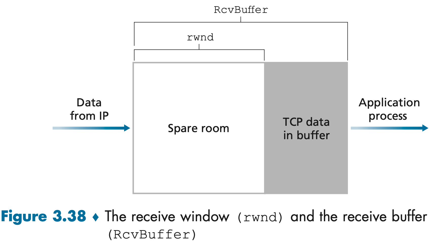
TCP provides flow control by having the sender maintain a variable called the receive window: rwnd = RcvBuffer – [LastByteRcvd – LastByteRead]

Host A makes sure throughout the connection’s life that, the amount of unacknowledged data that A has sent into the connection, less or equals than the rwnd: LastByteSent – LastByteAcked <= rwnd.

See interactive animation.

TCP Connection Management

Suppose a process running in one host (client) wants to initiate a connection with another process in another host (server):

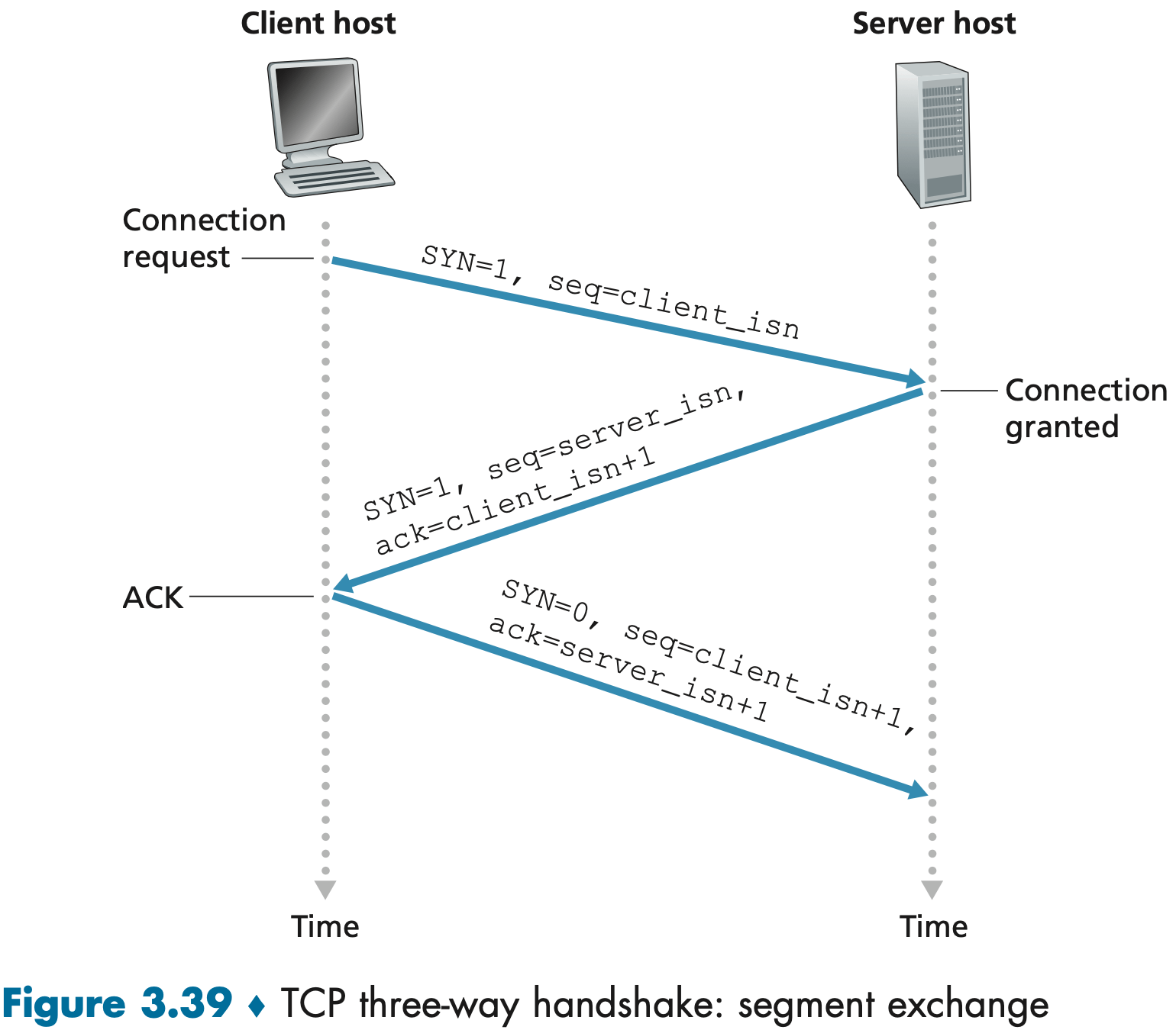
1. The client-side TCP first sends a special TCP segment, the SYN segment, to the server-side TCP. The SYN segment contains no application-layer data. But the SYN bit, is set to 1. In addition, the client randomly chooses an initial sequence number (client_isn) and puts this number in the sequence number field of the initial TCP SYN segment.
2. Once the TCP SYN segment arrives, the server allocates the TCP buffers and variables to the connection, and sends a connection-granted segment, the SYNACK segment, to the client TCP. The SYNACK segment also contains no application-layer data. However, it does contain three important pieces of information in the segment header. First, the SYN bit is set to 1. Second, the acknowledgment field of the TCP segment header is set to client_isn+1. Finally, the server chooses its own initial sequence number (server_isn) and puts this value in the sequence number field of the TCP segment header.
3. Upon receiving the SYNACK segment, the client also allocates buffers and variables to the connection. The client host then sends the server yet another segment, putting the value server_isn+1 in the acknowledgment field of the TCP segment header. The SYN bit is set to zero, since the connection is established. This third stage of the three-way handshake may carry client-to-server data in the segment payload.

Once these three steps have been completed, the client and server hosts can send segments containing data to each other.

Either of the two processes participating in a TCP connection can end the connection. suppose the client decides to close the connection:

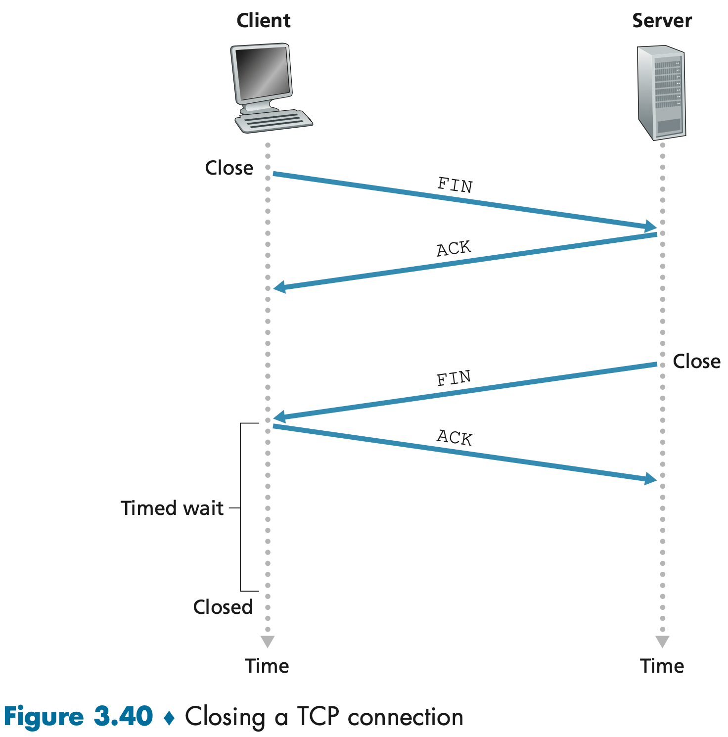
• The client TCP sends a TCP segment with the FIN bit set to 1.（之后客户端停止发送数据，但仍会对收到的数据进行确认）
• When the server receives this segment, it sends the client an acknowledgment segment in return.（此时服务端还可能继续发送一些数据，客户端也会对这些数据返回 ACK 确认）
• The server then sends its own shutdown segment, which has the FIN bit set to 1.（之后服务端也停止发送数据）
• The client acknowledges the server’s shutdown segment and wait for a time, typically 30 seconds, letting the TCP client resend the final acknowledgment in case the ACK is lost. After the wait, the connection formally closes and all resources on the client side (including port numbers) are released.
• The server receives the final ACK and closes down.

TCP 关闭连接时，主动方和被动方分别发生了什么：

• 双方都需要发送 FIN 信号，并且，发送 ACK 以确认对方发的 FIN 信号
• 主动方在发送最后的 ACK 后，需要等待 2MSL 的时间，这是为了确认被动方收到了最后的 ACK

The MSL is the maximum amount of time that a TCP segment can live in the network.

Nmap ("Network Mapper") is a free and open source (license) utility for network discovery and security auditing.

Classic TCP Congestion Control (TCP Reno)

TCP 拥塞控制的方法是让每一个发送方根据所感知到的网络拥塞程度来限制其发送流量的速率。

The TCP congestion-control mechanism operating at the sender keeps track of an additional variable, the congestion window, denoted cwnd. Specifically, the amount of unacknowledged data at a sender may not exceed the minimum of cwnd and rwnd, that is: LastByteSent – LastByteAcked <= min{cwnd, rwnd}.（TCP 流水线中可以同时发送的、即未经 ACK 确认的数据量，不能超过拥塞窗口和接收窗口中的较小值）

The constraint above limits the amount of unacknowledged data at the sender and therefore indirectly limits the sender’s send rate.

There is no explicit signaling of congestion state by the network—ACKs and loss events serve as implicit signals. The loss event at the sender—either a timeout or the receipt of three duplicate ACKs (totally 4 ACKs)—which is taken by the sender to be an indication of congestion on the sender-to-receiver path. An acknowledged segment indicates that the network is delivering the sender’s segments to the receiver, and hence, the sender’s rate can be increased when an ACK arrives.

We’re now in a position to consider the details of the celebrated TCP congestion-control algorithm, which has three major components: (1) slow start, (2) congestion avoidance, and (3) fast recovery.

In the slow-start state, the value of cwnd begins at 1 MSS and increases by 1 MSS every time a transmitted segment is first acknowledged. This process results in a doubling of the sending rate every RTT. Thus, the TCP send rate starts slow but grows exponentially during the slow start phase.

• Timeout: ssthresh = cwnd/2; cwnd = 1 MSS;, begins the slow start process anew.
• 3 duplicate ACKs: ssthresh = cwnd/2; cwnd = ssthresh + 3 * MSS;, performs a fast retransmit and enters the fast recovery state.
• When cwnd == ssthresh, slow start ends and TCP transitions into congestion avoidance mode.

On entry to the congestion-avoidance state, TCP linearly increases the value of cwnd by just a single MSS every RTT.

• Timeout: ssthresh = cwnd/2; cwnd = 1 MSS;, begins the slow start process anew.
• 3 duplicate ACKs: ssthresh = cwnd/2; cwnd = ssthresh + 3 * MSS;, performs a fast retransmit and enters the fast recovery state.

In fast recovery state, the value of cwnd is increased by 1 MSS for every duplicate ACK received for the missing segment. Eventually, when an ACK arrives for the missing segment, TCP enters the congestion-avoidance state and sets cwnd = ssthresh.

• Timeout: ssthresh = cwnd/2; cwnd = 1 MSS;, begins the slow start process anew.

[1] ssthresh: slow start threshold.

[2] Adding in 3 MSS for good measure to account for the triple duplicate ACKs received. This artificially "inflates" the congestion window by the number of segments (three) that have left the network and which the receiver has buffered [RFC 2582].

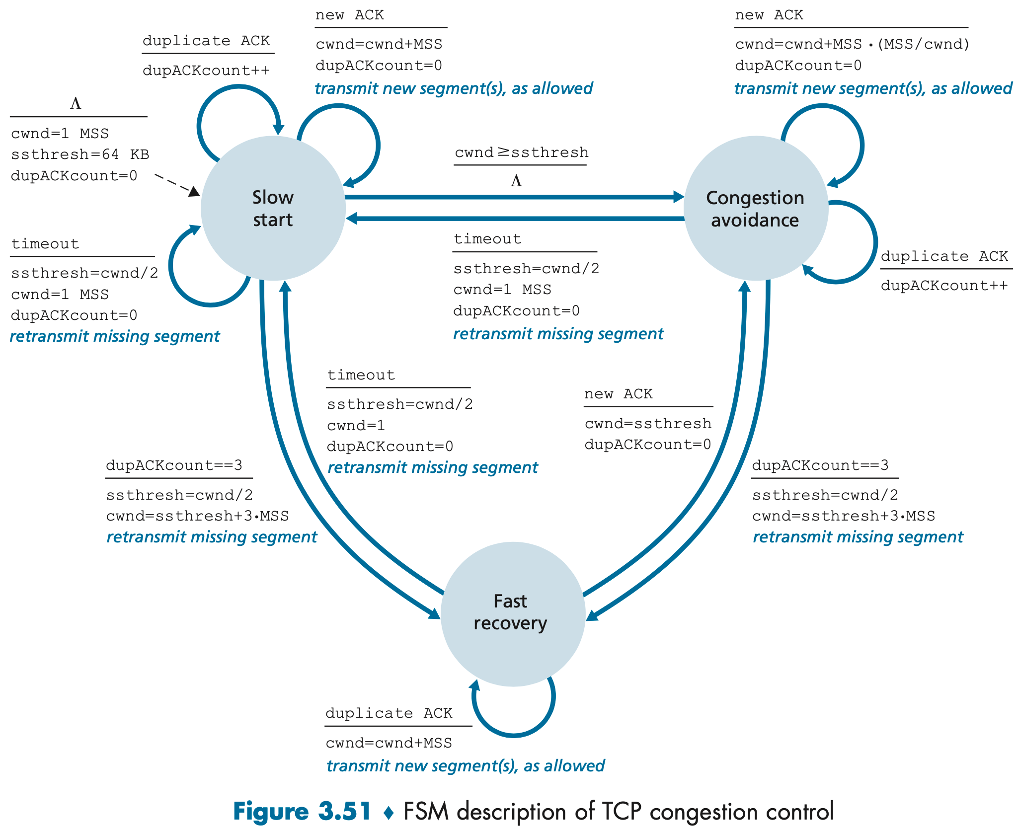
The arrows in the FSM description indicate the transition of the protocol from one state to another.

The event causing the transition is shown above the horizontal line labeling the transition, and the actions taken when the event occurs are shown below the horizontal line.

When no action is taken on an event, or no event occurs and an action is taken, we’ll use the symbol Λ below or above the horizontal, respectively, to explicitly denote the lack of an action or event.

The initial state of the FSM is indicated by the dashed arrow.

Ignoring the slow-start phase (This phase is typically very short, since the sender grows out of the phase exponentially fast) and assuming that losses are indicated by triple duplicate ACKs, TCP’s congestion control consists of linear (additive) increase in cwnd of 1 MSS per RTT and then a halving (multiplicative decrease) of cwnd on a triple duplicate-ACK event. For this reason, TCP congestion control is often referred to as an additive-increase, multiplicative-decrease (AIMD) form of congestion control.

TCP Reno’s AIMD to congestion control may be overly cautious. It’s better to more quickly ramp up the sending rate to get close to the pre-loss sending rate and only then probe cautiously for bandwidth. This insight lies at the heart of a flavor of TCP known as TCP CUBIC, who has recently gained wide deployment.

Explicit Congestion Notification and Delayed-based Congestion Control

TCP 拥塞控制已经演化了多年并仍在继续演化。

More recently, extensions to both IP and TCP [RFC 3168] have been proposed, implemented, and deployed that allow the network to explicitly signal congestion to a TCP sender and receiver.

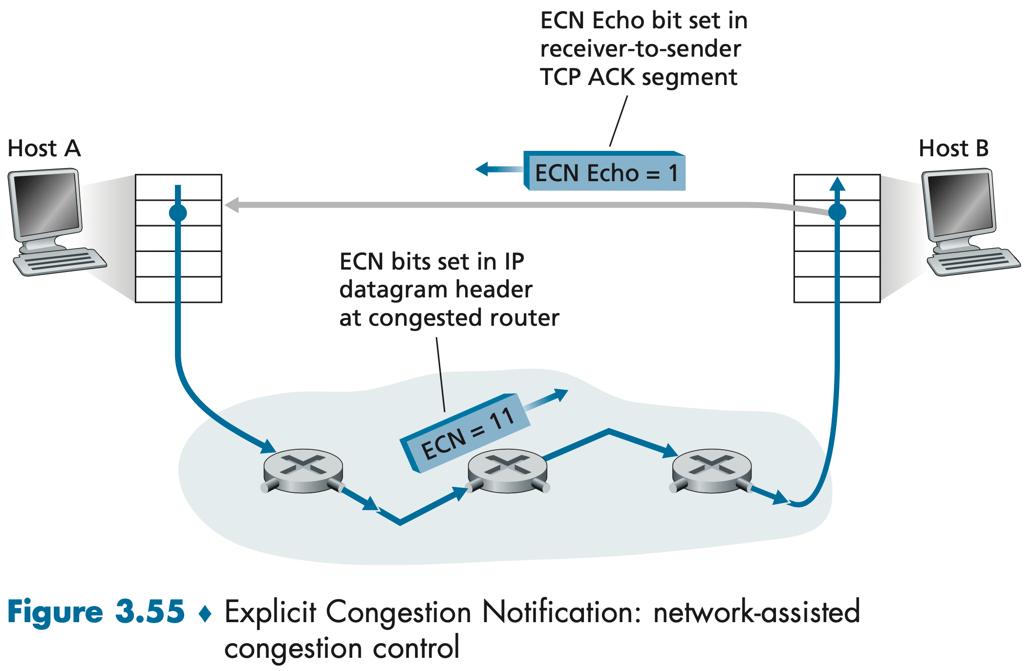
Explicit Congestion Notification (ECN) 显式阻塞通知 is the form of network-assisted congestion control performed within the Internet. Both TCP and IP are involved. At the network layer, two bits (with four possible values, overall) in the "Type of Service field" of the IP datagram header are used for ECN.

One setting of the ECN bits is used by a router to indicate that it (the router) is experiencing congestion. A second setting of the ECN bits is used by the sending host to inform routers that the sender and receiver are ECN-capable, and thus capable of taking action in response to ECN-indicated network congestion.

The intuition is that the congestion indication bit can be set to signal the onset of congestion to the sender before loss actually occurs.

As shown in Figure 3.55, when the TCP in the receiving host receives an ECN congestion indication via a received IP datagram, the TCP in the receiving host informs the TCP in the sending host of the congestion indication by setting the ECE (Explicit Congestion Notification Echo) bit in a receiver-to-sender TCP ACK segment. The TCP sender, in turn, reacts by halving the congestion window, as it would react to a lost segment using fast retransmit, and sets the CWR (Congestion Window Reduced) bit in the header of the next transmitted TCP sender-to-receiver segment.

In addition, a number of variations of TCP congestion control protocols have been proposed that infer congestion using measured packet delay.

Fairness

TCP 的 AIMD 算法公平吗? TCP 趋于在竞争的多条 TCP 连接之间提供对瓶颈链路带宽的平等分享。但实践中，那些具有较小 RTT 的连接能够通过更快地增大其拥塞窗口、抢到更多的可用带宽，因而比那些具有较大 RTT 的连接享用更高的吞吐量。

UDP 是没有内置的拥塞控制的。实时通话应用通常希望以恒定的速率将其数据注入网络，它们可以接受偶尔丢失分组，但不愿在拥塞时将其发送速率降至“公平”级别而不丢失任何分组。从 TCP 的观点来看，运行在 UDP 上的应用是不公平的，因为它们不与其他连接合作、适时地调整传输速率，UDP 有可能压制 TCP 流量。当今的一个主要研究领域就是因特网的拥塞控制机制，用于阻止 UDP 流量不断压制直至中断因特网吞吐量的情况。

即使我们能够使 UDP 流量具有公平的行为，但公平性问题仍然没有完全解决。因为我们没有办法阻止应用使用多个并行 TCP 连接。例如，Web 浏览器通常使用多个并行 TCP 连接来传送一个 Web

Evolution

Three decades of experience with TCP and UDP has identified circumstances in which neither is ideally suited, and so the design and implementation of transport layer functionality has continued to evolve.

Indeed, measurements in [Yang 2014] indicate that CUBIC (and its predecessor, BIC [Xu 2004]) and CTCP are more widely deployed on Web servers than classic TCP Reno; we also saw that BBR is being deployed in Google’s internal B4 network, as well as on many of Google’s public-facing servers. And there are many (many!) more versions of TCP!

QUIC is a new application-layer protocol designed from the ground up to improve the performance of transport-layer services for secure HTTP. QUIC has already been widely deployed, although is still in the process of being standardized as an Internet RFC.

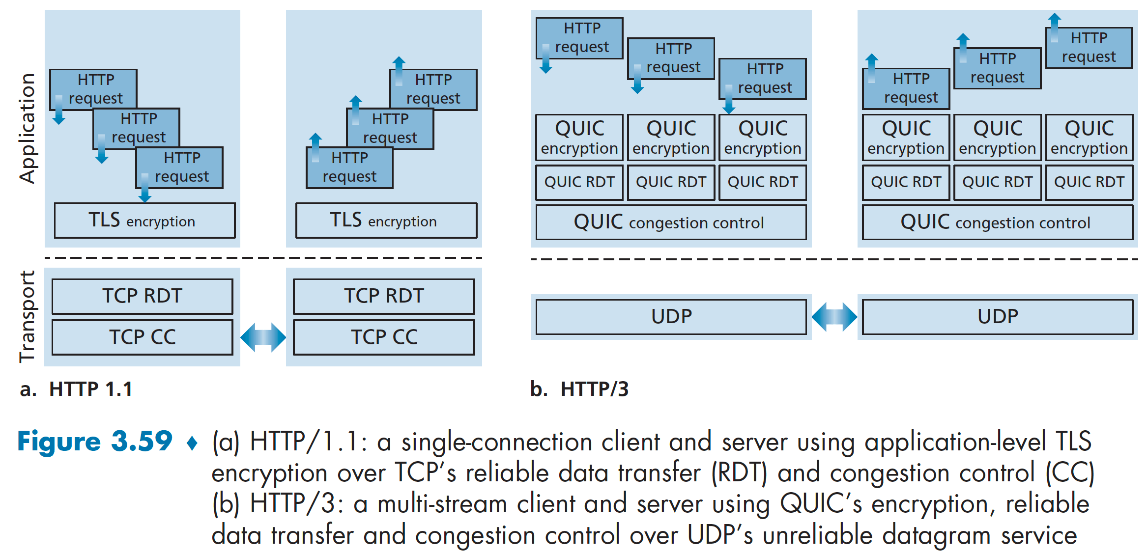
QUIC is an application-layer protocol, using UDP as its underlying transport-layer protocol, and is designed to interface above specifically to a simplified but evolved version of HTTP/2. In the near future, HTTP/3 will natively incorporate QUIC.

Some of QUIC’s major features include:

• Connection-Oriented and Secure. QUIC combines the handshakes needed to establish connection state with those needed for authentication and encryptionm, thus providing faster establishment.
• Streams. QUIC allows several different application-level “streams” to be multiplexed through a single QUIC connection. Data from multiple streams may be contained within a single QUIC segment, which is carried over UDP.
• Reliable, TCP-friendly congestion-controlled data transfer. QUIC provides reliable data transfer to each QUIC stream separately. Since QUIC provides a reliable in-order delivery on a per-stream basis, a lost UDP segment only impacts those streams whose data was carried in that segment; HTTP messages in other streams can continue to be received and delivered to the application. QUIC provides reliable data transfer using acknowledgment mechanisms similar to TCP’s, as specified in [RFC 5681].

Network Layer

Having now covered the application layer and the transport layer, our discussion of the network edge is complete. It is time to explore the network core!

The network layer is arguably the most complex layer in the protocol stack. We’ll see that the network layer can be decomposed into two interacting parts, the data plane and the control plane.

In Chapter 4, we’ll first cover the data plane functions—the per-router functions that determine how a datagram arriving on one of a router’s input links is forwarded to one of that router’s output links.

In Chapter 5, we’ll cover the control plane functions—the network-wide logic that controls how a datagram is routed among routers along an end-to-end path from the source host to the destination host, also, how network-layer components and services are configured and managed.

Forwarding refers to the router-local action of transferring a packet from an input link interface to the appropriate output link interface. Forwarding takes place at very short timescales (typically a few nanoseconds), and thus is typically implemented in hardware.

Routing refers to the network-wide process that determines the end-to-end paths that packets take from source to destination. Routing takes place on much longer timescales (typically seconds), and as we will see is often implemented in software.

Some packet switches, called link-layer switches, base their forwarding decision on values in the fields of the link-layer frame; switches are thus referred to as link-layer (layer 2) devices. Other packet switches, called routers, base their forwarding decision on header field values in the network-layer datagram. Routers are thus network-layer (layer 3) devices.

Data Plane

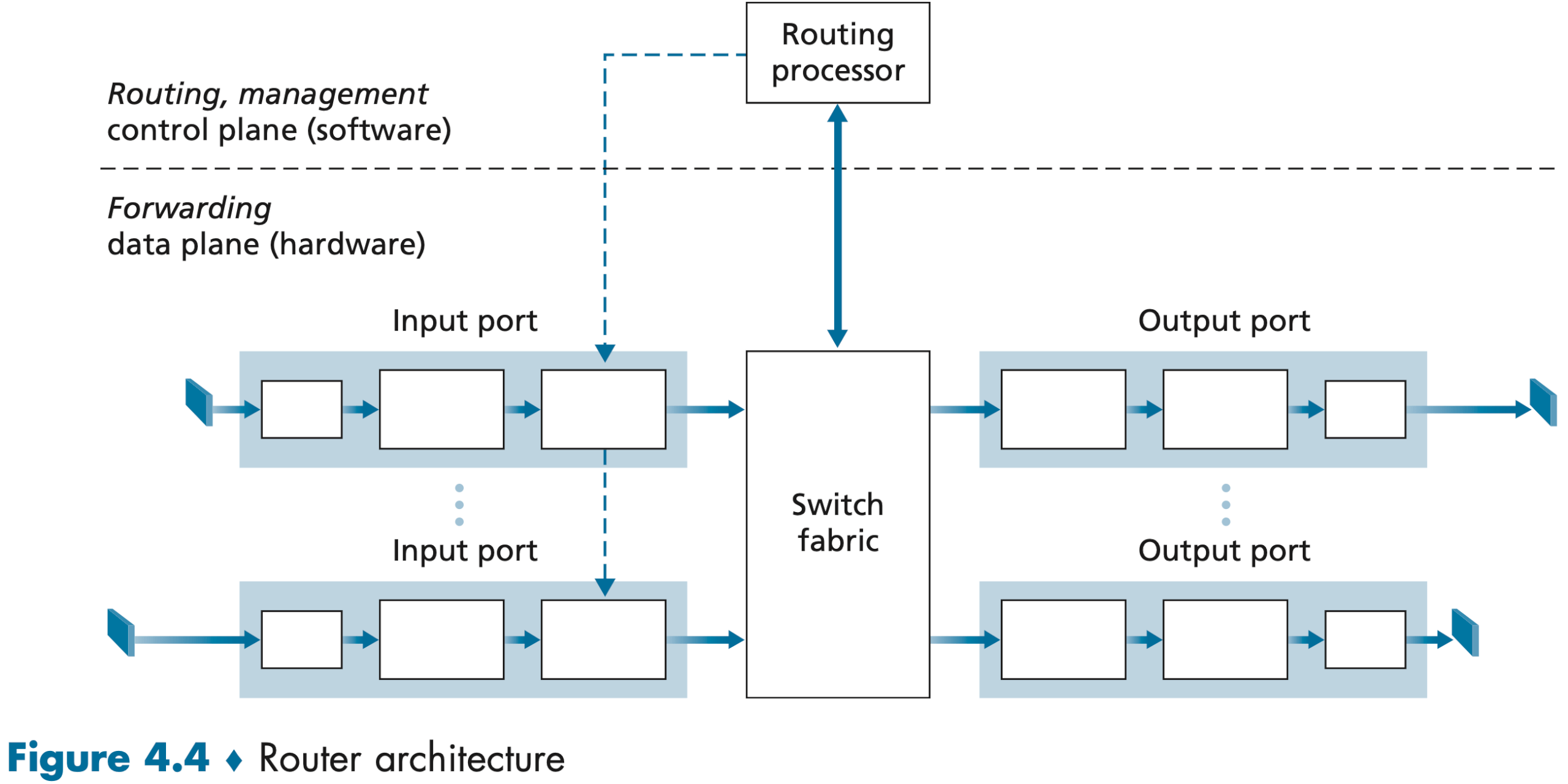
Router

一台路由器的组成：（注意这里的端口指的是物理硬件端口，而非软件端口）

• Input ports. It is here that the forwarding table is consulted to determine the router output port to which an arriving packet will be forwarded via the switching fabric. Control packets (for example, packets carrying routing protocol information) are forwarded from an input port to the routing processor.
• Switching fabric. The switching fabric connects the router’s input ports to its output ports. A network inside of a router!
• Output ports. An output port stores packets received from the switching fabric and transmits these packets on the outgoing link.
• Routing processor. The routing processor performs control-plane functions. In traditional routers, it executes the routing protocols, maintains routing tables and attached link state information, and computes the forwarding table for the router. In SDN routers, the routing processor is responsible for communicating with the remote controller in order to (among other activities) receive forwarding table entries computed by the remote controller, and install these entries in the router’s input ports.

A router’s input ports, output ports, and switching fabric are almost always implemented in hardware.

The lookup performed in the input port is central to the router’s operation—it is here that the router uses the forwarding table to look up the output port to which an arriving packet will be forwarded via the switching fabric.

The forwarding table is either computed and updated by the routing processor (using a routing protocol to interact with the routing processors in other network routers, the traditional approach) or is received from a remote SDN controller (The SDN approach).

We’ll initially assume in this section that forwarding decisions are based only on the packet’s destination address, rather than on a generalized set of packet header fields. The router matches a prefix of the packet’s destination address with the entries in the table; When there are multiple matches, the router uses the longest prefix matching rule.

Prefix	Link Interface
11001000 00010111 00010	0
11001000 00010111 00011000	1
11001000 00010111 00011	2
Otherwise	3

Once a packet’s output port has been determined via the lookup, the packet can be sent into the switching fabric.

Switching can be accomplished in a number of ways: Switching via memory; Switching via a bus; Switching via an interconnection network.

If the switch fabric is not fast enough (relative to the input line speeds) to transfer all arriving packets through the fabric without delay, packet queuing can occur at the input ports.

Output port processing takes packets that have been stored in the output port’s memory and transmits them over the output link. This includes selecting and de-queueing packets for transmission, and performing the needed link-layer and physical-layer transmission functions.

IPv4

Note that an IP datagram has a total of 20 bytes of header (assuming no options). If the datagram carries a TCP segment, then each datagram carries a total of 40 bytes of header (20 bytes of IP header plus 20 bytes of TCP header) along with the application-layer message.

A host typically has only a single link into the network. The boundary between the host and the physical link is called an interface. The boundary between the router and any one of its links is also called an interface. A router thus has multiple interfaces, one for each of its links. Because every host and router is capable of sending and receiving IP datagrams, IP requires each host and router interface to have its own IP address. Thus, an IP address is technically associated with an interface, rather than with the host or router containing that interface.

Each IP address is 32 bits long (4 bytes), and there are thus a total of 2 ^ 32 (or approximately 4 billion) possible IP addresses.

Each interface on every host and router in the global Internet must have an IP address that is globally unique (except for interfaces behind NATs).

Figure 4.18 provides an example of IP addressing and interfaces.

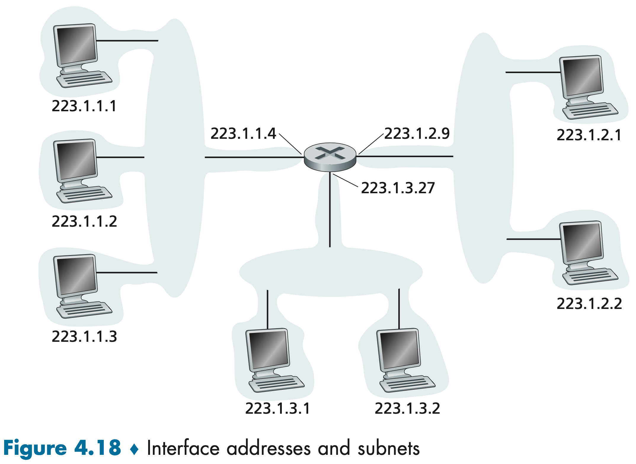
The three hosts in the upper-left portion of Figure 4.18, and the router interface to which they are connected, all have an IP address of the form 223.1.1.xxx. In IP terms, this network interconnecting three host interfaces and one router interface forms a subnet. IP addressing assigns an address to this subnet: 223.1.1.0/24, where the /24 notation, sometimes known as a subnet mask 子网掩码, indicates that the leftmost 24 bits of the 32-bit quantity define the subnet address. Any additional hosts attached to the 223.1.1.0/24 subnet would be required to have an address of the form 223.1.1.xxx.

It’s clear that an organization (such as a company or academic institution) with multiple Ethernet segments and point-to-point links will have multiple subnets, with all of the devices on a given subnet having the same subnet address.

The global Internet’s address assignment strategy is known as Classless Interdomain Routing (CIDR—pronounced cider) [RFC 4632]. CIDR generalizes the notion of subnet addressing. As with subnet addressing, the 32-bit IP address is divided into two parts and again has the dotted-decimal form a.b.c.d/x, where x indicates the number of bits in the first part of the address.

An organization is typically assigned a block of contiguous addresses, that is, a range of addresses with a common prefix. In this case, the IP addresses of devices within the organization will share the common prefix.

The remaining 32 - x bits of an address can be thought of as distinguishing among the devices within the organization, all of which have the same network prefix. These are the bits that will be considered only when forwarding packets at routers within the organization. These lower-order bits may (or may not) have an additional subnetting structure. （组织内部又可以分割成更多的子网）

IP broadcast address: When a host sends a datagram with destination address 255.255.255.255, the message is delivered to all hosts on the same subnet (e.g. using in DHCP).

Let’s begin looking at how an organization gets a block of addresses for its devices, and then look at how a device (such as a host) is assigned an address from within the organization’s block of addresses.

In order to obtain a block of IP addresses for use within an organization’s subnet, a network administrator might first contact its ISP, which would provide addresses from a larger block of addresses that had already been allocated to the ISP.

Is there a global authority that has ultimate responsibility for managing the IP address space and allocating address blocks to ISPs and other organizations? IP addresses are managed under the authority of the ICANN. The role of the nonprofit ICANN organization is not only to allocate IP addresses, but also to manage the DNS root servers.

Once an organization has obtained a block of addresses, it can assign individual IP addresses to the host and router interfaces in its organization. Typically this is done using the Dynamic Host Configuration Protocol (DHCP). DHCP allows a host to obtain (be allocated) an IP address automatically. A network administrator can configure DHCP so that a given host receives the same IP address each time it connects to the network, or a host may be assigned a temporary IP address that will be different each time the host connects to the network. In addition to host IP address assignment, DHCP also allows a host to learn additional information, such as its subnet mask, the address of its first-hop router (often called the default gateway), and the address of its local DNS server.

DHCP is a client-server protocol. A client is typically a newly arriving host wanting to obtain network configuration information, including an IP address for itself. In the simplest case, each subnet will have a DHCP server. If no server is present on the subnet, a DHCP relay agent (typically a router) that knows the address of a DHCP server for that network is needed.

For a newly arriving host, the DHCP protocol is a four-step process: DHCP server discovery; DHCP server offer(s); DHCP request; DHCP ACK.

NAT

The address space 10.0.0.0/8 is one of three portions of the IP address space that is reserved in [RFC 1918] for a private network. The other two are 172.16.0.0/12, 192.168.0.0/16.

Figure 4.25 shows the operation of Network Address Translation (NAT). The NAT-enabled router, residing in the home, has an interface that is part of the home network on the right of Figure 4.25.

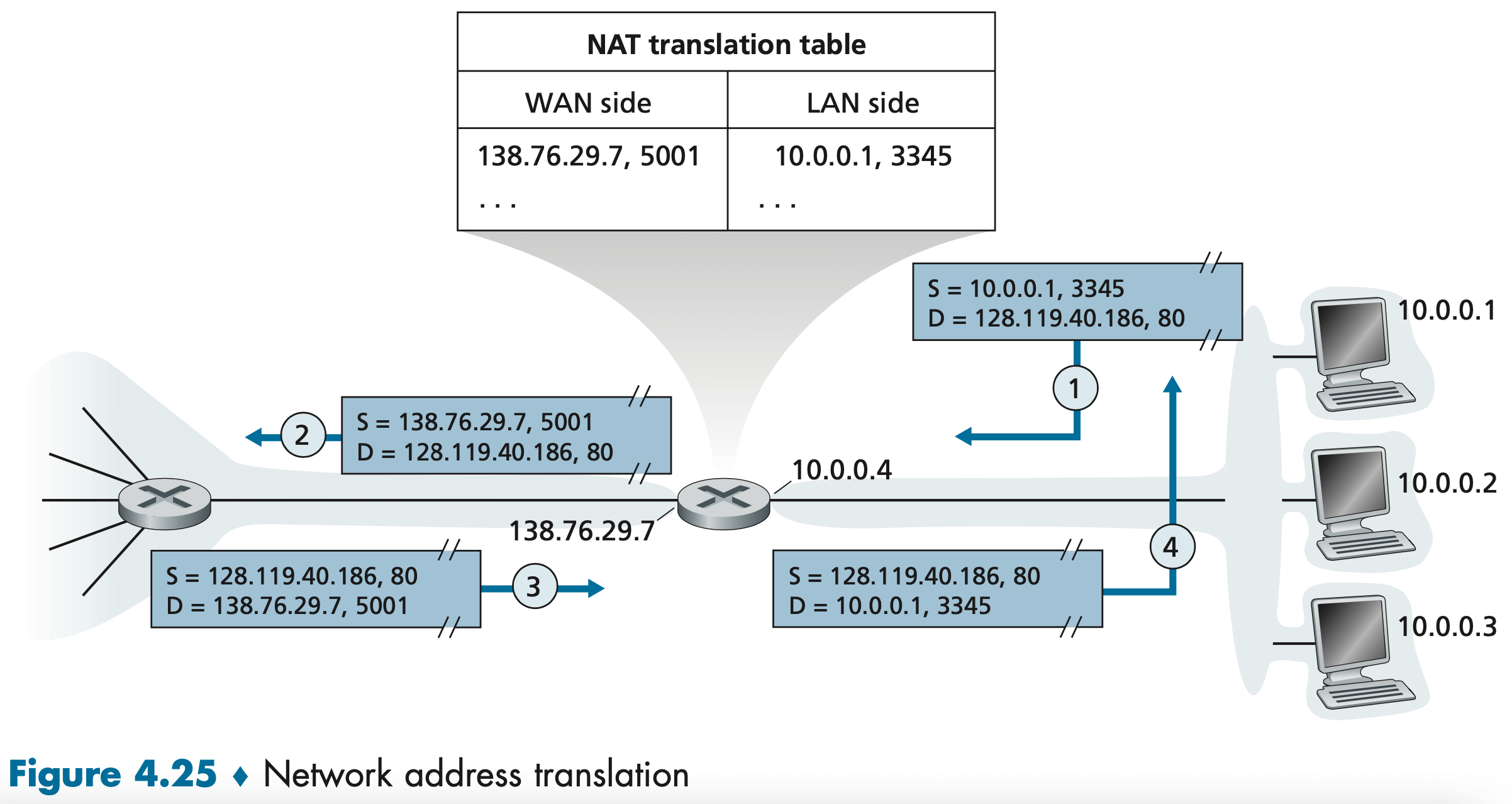
The NAT router behaves to the outside world as a single device with a single IP address. The router gets its address from the ISP’s DHCP server, and the router runs a DHCP server to provide addresses to computers within the NAT-DHCP-router-controlled home network’s address space.

If all datagrams arriving at the NAT router from the WAN (Wide area network) have the same destination IP address, then how does the router know the internal host to which it should forward a given datagram? The trick is to use a NAT translation table at the NAT router, and to include port numbers as well as IP addresses in the table entries.

IPv6

In the early 1990s, the Internet Engineering Task Force began an effort to develop a successor to the IPv4 protocol. A prime motivation for this effort was the realization that the 32-bit IPv4 address space was beginning to be used up.

The most important changes introduced in IPv6 are evident in the datagram format: IPv6 increases the size of the IP address from 32 to 128 bits. This ensures that the world won’t run out of IP addresses.

How will the public Internet, which is based on IPv4, be transitioned to IPv6? The problem is that while new IPv6-capable systems can be made backward-compatible, that is, can send, route, and receive IPv4 datagrams, already deployed IPv4-capable systems are not capable of handling IPv6 datagrams.

The approach to IPv4-to-IPv6 transition that has been most widely adopted in practice involves tunneling.

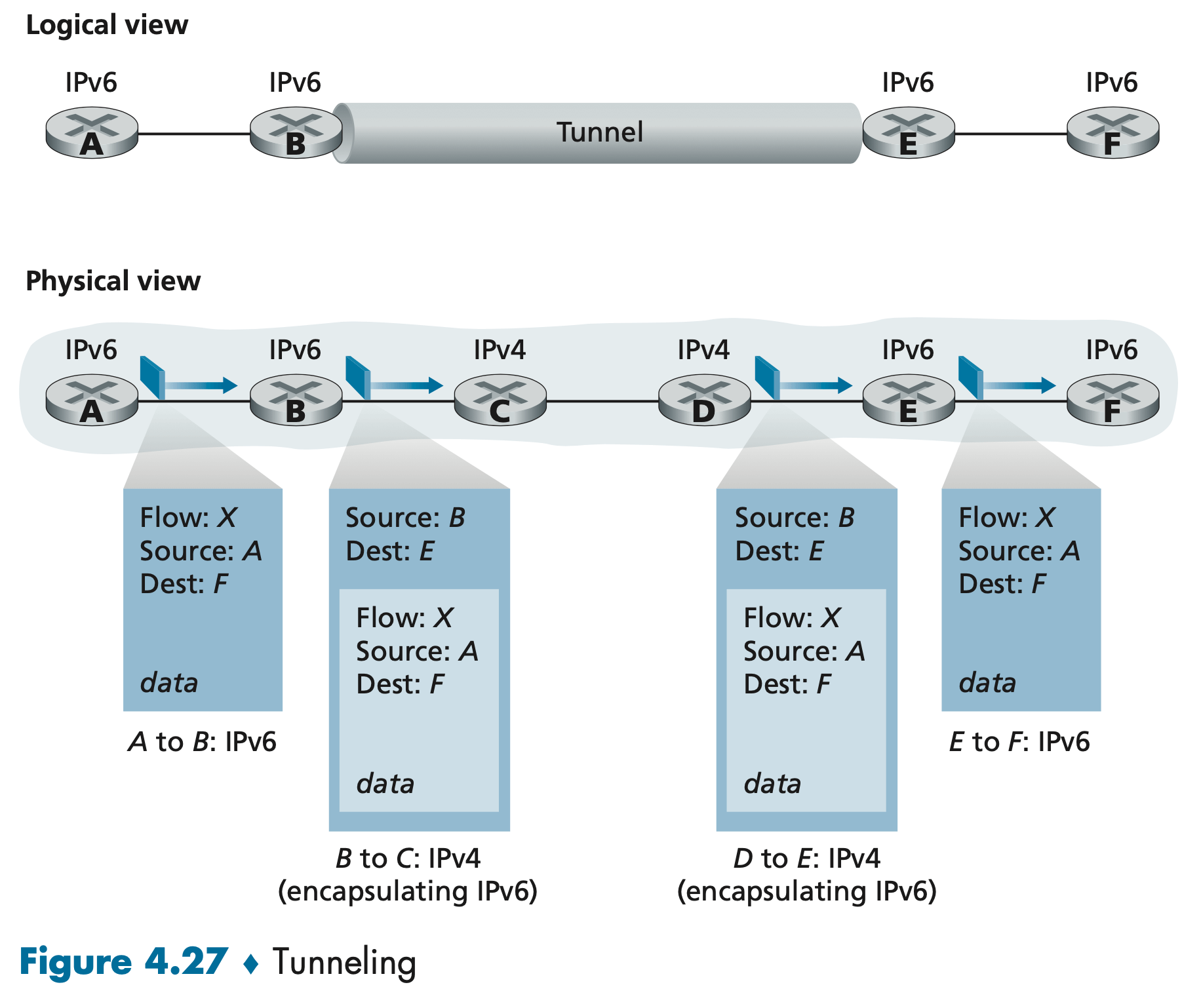
Suppose two IPv6 nodes (in this example, B and E in Figure 4.27) want to interoperate using IPv6 datagrams but are connected to each other by intervening IPv4 routers. We refer to the intervening set of IPv4 routers between two IPv6 routers as a tunnel. With tunneling, the IPv6 node on the sending side of the tunnel (in this example, B) takes the entire IPv6 datagram and puts it in the data (payload) field of an IPv4 datagram. This IPv4 datagram is then addressed to the IPv6 node on the receiving side of the tunnel (in this example, E) and sent to the first node in the tunnel (in this example, C). The intervening IPv4 routers in the tunnel route this IPv4 datagram among themselves, just as they would any other datagram. The IPv6 node on the receiving side determines that the payload is a IPv6 datagram, extracts the IPv6 datagram, and then routes the IPv6 datagram exactly as it would if it had received the IPv6 datagram from a directly connected IPv6 neighbor.

Control Plane

We saw that the forwarding table (in the case of destination-based forwarding) and the flow table (in the case of generalized forwarding) were the principal elements that linked the network layer’s data and control planes. We saw that in the case of generalized forwarding, the actions taken could include not only forwarding a packet to a router’s output port, but also dropping a packet, replicating a packet, and/or rewriting layer 2, 3 or 4 packet-header fields.

In this chapter, we’ll study how those forwarding and flow tables are computed, maintained and installed. We learned that there are two possible approaches for doing so:

• Per-router control: Each router has a routing component that communicates with the routing components in other routers to compute the values for its forwarding table. This per-router control approach has been used in the Internet for decades. The OSPF and BGP are based on this per-router approach to control.
• Software-defined networking (SDN) control: A logically centralized controller computes and distributes the forwarding tables to be used by each and every router. The OpenFlow protocol operates between an SDN controller and an SDN-controlled switch or other device implementing the OpenFlow API. The OpenFlow protocol operates over TCP, with a default port number of 6653.

Routing Algorithms

The goal of routing algorithms is to determine the least cost paths (equivalently, routes), from senders to receivers, through the network of routers. A graph is used to formulate routing problems. The least-cost problem is therefore clear: Find a path between the source and destination that has least cost. Note that if all edges in the graph have the same cost, the least-cost path is also the shortest path (that is, the path with the smallest number of links between the source and the destination).

A centralized routing algorithm computes the least-cost path using complete, global knowledge about the network. Algorithms with global state information are often referred to as link-state (LS) algorithms, since the algorithm must be aware of the cost of each link in the network. In practice, this is accomplished by having each node broadcast link-state packets to all other nodes in the network, with each link-state packet containing the identities and costs of its attached links. In practice (for example, with the Internet’s OSPF routing protocol), this is often accomplished by a link-state broadcast algorithm. The result of the nodes’ broadcast is that all nodes have an identical and complete view of the network. Each node can then run the LS algorithm and compute the same set of least-cost paths as every other node.

In a decentralized routing algorithm, the calculation of the least-cost path is carried out in an iterative, distributed manner by the routers. No node has complete information about the costs of all network links. Instead, each node begins with only the knowledge of the costs of its own directly attached links. Then, through an iterative process of calculation and exchange of information with its neighboring nodes, a node gradually calculates the least-cost path to a destination or set of destinations. The decentralized routing algorithm we’ll study is called a distance-vector (DV) algorithm, because each node maintains a vector of estimates of the costs (distances) to all other nodes in the network. Such decentralized algorithms, with interactive message exchange between neighboring routers is perhaps more naturally suited to control planes where the routers interact directly with each other.

Neither algorithm is an obvious winner over the other; indeed, both algorithms are used in the Internet. These two algorithms are the basis for two widely deployed Internet routing protocols, OSPF and BGP.

OSPF and BGP

In our study of routing algorithms, we’ve viewed the network simply as a collection of interconnected routers. In practice, this model is simplistic for two important reasons: First, today’s Internet consists of hundreds of millions of routers. Storing routing information for possible destinations at each of these routers would clearly require enormous amounts of memory. The overhead required to broadcast connectivity and link cost updates among all of the routers would be huge! A distance-vector algorithm that iterated among such a large number of routers would surely never converge. Clearly, something must be done to reduce the complexity of route computation in a network as large as the Internet. Second, the Internet is a network of ISPs, with each ISP consisting of its own network of routers. An ISP generally desires to operate its network as it pleases or to hide aspects of its network’s internal organization from the outside. Ideally, an organization should be able to operate and administer its network as it wishes, while still being able to connect its network to other outside networks.

Both of these problems can be solved by organizing routers into autonomous systems (ASs), with each AS consisting of a group of routers that are under the same administrative control. An autonomous system is identified by its globally unique autonomous system number (ASN). AS numbers, like IP addresses, are assigned by ICANN regional registries.

Routers within the same AS all run the same routing algorithm and have infor- mation about each other. The routing algorithm running within an autonomous sys- tem is called an intra-autonomous system routing protocol. OSPF routing and its closely related cousin, IS-IS, are widely used for intra-AS routing in the Internet.

Since an inter-AS routing protocol involves coordination among multiple ASs, communicating ASs must run the same inter-AS routing protocol. In fact, in the Internet, all ASs run the same inter-AS routing protocol, called the Border Gateway Protocol, more commonly known as BGP.

Managing the IP Network

The Internet Control Message Protocol (ICMP), specified in [RFC 792], is used by hosts and routers to communicate network-layer information to each other.

In practice, there are three commonly used ways in a network operator can manage the network:

• CLI. A network operator may issue direct Command Line Interface (CLI) commands to the device. These commands can be typed directly on a managed device’s console (if the operator is physically present at the device), or over a Telnet or secure shell (SSH) connection, possibly via scripting, between the managing server/controller and the managed device.
• SNMP/MIB. In this approach, the network operator can query/set the data contained in a device’s Management Information Base (MIB) objects using the Simple Network Management Protocol (SNMP).
• NETCONF/YANG. The NETCONF/YANG approach takes a more abstract, network-wide, and holistic view toward network management, with a much stronger emphasis on configuration management, including specifying correctness constraints and providing atomic management operations over multiple controlled devices. YANG [RFC 6020] is a data modeling language used to model configuration and operational data. The NETCONF protocol [RFC 6241] is used to communicate YANG-compatible actions and data to/from/among remote devices.

Link Layer

We refer to any device that runs a link-layer protocol as a node. Nodes include hosts, routers, switches, and WiFi access points. We will also refer to the communication channels that connect adjacent nodes along the communication path as links.

The basic service of the link layer is to move a network-layer datagram from one node to an adjacent node.

In order for a datagram to be transferred from source host to destination host, it must be moved over each of the individual links in the end-to-end path. Over a given link, a transmitting node encapsulates the datagram in a link-layer frame and transmits the frame into the link.

There are two types of network links: point-to-point links and broadcast links.

A point-to-point link consists of a single sender at one end of the link and a single receiver at the other end of the link. The point-to-point protocol (PPP) and high-level data link control (HDLC) are two protocols designed for point-to-point links.

A broadcast link, can have multiple sending and receiving nodes all connected to the same, single, shared broadcast channel. The term broadcast is used here because when any one node transmits a frame, the channel broadcasts the frame and each of the other nodes receives a copy. Ethernet and wireless LANs are examples of broadcast link-layer technologies.

Multiple Access Protocols

A problem of central importance to the link layer: how to coordinate the access of multiple sending and receiving nodes to a shared broadcast channel—the multiple access problem. Computer have so-called multiple access protocols by which nodes regulate their transmission into the shared broadcast channel. We can classify them to one of three categories: channel partitioning protocols, random access protocols, and taking-turns protocols.

Channel Partitioning Protocols

Time-division multiplexing (TDM) divides time into time frames and further divides each time frame into N time slots. Each time slot is then assigned to one of the N nodes. Whenever a node has a packet to send, it transmits the packet’s bits during its assigned time slot in the revolving TDM frame. TDM is appealing because it eliminates collisions and is perfectly fair. However, it has two major drawbacks. First, a node is limited to an average rate of R/N bps even when it is the only node with packets to send. A second drawback is that a node must always wait for its turn in the transmission sequence—again, even when it is the only node with a frame to send.

Frequency-division multiplexing (FDM) divides the R bps channel into different frequencies (each with a bandwidth of R/N) and assigns each frequency to one of the N nodes. It avoids collisions and divides the bandwidth fairly among the N nodes. However, FDM also shares a principal disadvantage with TDM—a node is limited to a bandwidth of R/N, even when it is the only node with packets to send.

Code division multiple access (CDMA) assigns a different code to each node. Each node then uses its unique code to encode the data bits it sends. If the codes are chosen carefully, CDMA networks have the wonderful property that different nodes can transmit simultaneously.

Random Access protocols

In a random access protocol, a transmitting node always transmits at the full rate of the channel, namely, R bps. When there is a collision, each node involved in the collision repeatedly retransmits its frame (that is, packet) until its frame gets through without a collision. But when a node experiences a collision, it doesn’t necessarily retransmit the frame right away. Instead it waits a random delay before retransmitting the frame. Each node involved in a collision chooses independent random delays. Because the random delays are independently chosen, it is possible that one of the nodes will pick a delay that is sufficiently less than the delays of the other colliding nodes and will therefore be able to sneak its frame into the channel without a collision.

A few of the most commonly used random access protocols—the ALOHA protocols and the carrier sense multiple access (CSMA) protocols. Ethernet is a popular and widely deployed CSMA protocol.

Taking-Turns Protocols

The first one is the polling protocol. The polling protocol requires one of the nodes to be designated as a master node. The master node polls each of the nodes in a round-robin fashion. In particular, the master node first sends a message to node 1, saying that it (node 1) can transmit up to some maximum number of frames. After node 1 transmits some frames, the master node tells node 2 it (node 2) can transmit up to the maximum number of frames. (The master node can determine when a node has finished sending its frames by observing the lack of a signal on the channel.) The procedure continues in this manner, with the master node polling each of the nodes in a cyclic manner. The Bluetooth protocol is an example of a polling protocol.

The second one is the token-passing protocol. A small, special-purpose frame known as a token is exchanged among the nodes in some fixed order. When a node receives a token, it holds onto the token only if it has some frames to transmit; otherwise, it immediately forwards the token to the next node. If a node does have frames to transmit when it receives the token, it sends up to a maximum number of frames and then forwards the token to the next node. Token passing is decentralized and highly efficient. But it has its problems as well. For example, the failure of one node can crash the entire channel. Or if a node accidentally neglects to release the token, then some recovery procedure must be invoked to get the token back in circulation. Over the years many token-passing protocols have been developed, including the fiber distributed data interface (FDDI) protocol and the IEEE 802.5 token ring protocol, and each one had to address these as well as other sticky issues.

DOCSIS

A cable access network will make for an excellent case study here, as we’ll find aspects of each of these three classes of multiple access protocols with the cable access network! The Data-Over-Cable Service Interface Specifications (DOCSIS) specifies the cable data network architecture and its protocols.

Switched Local Area Networks

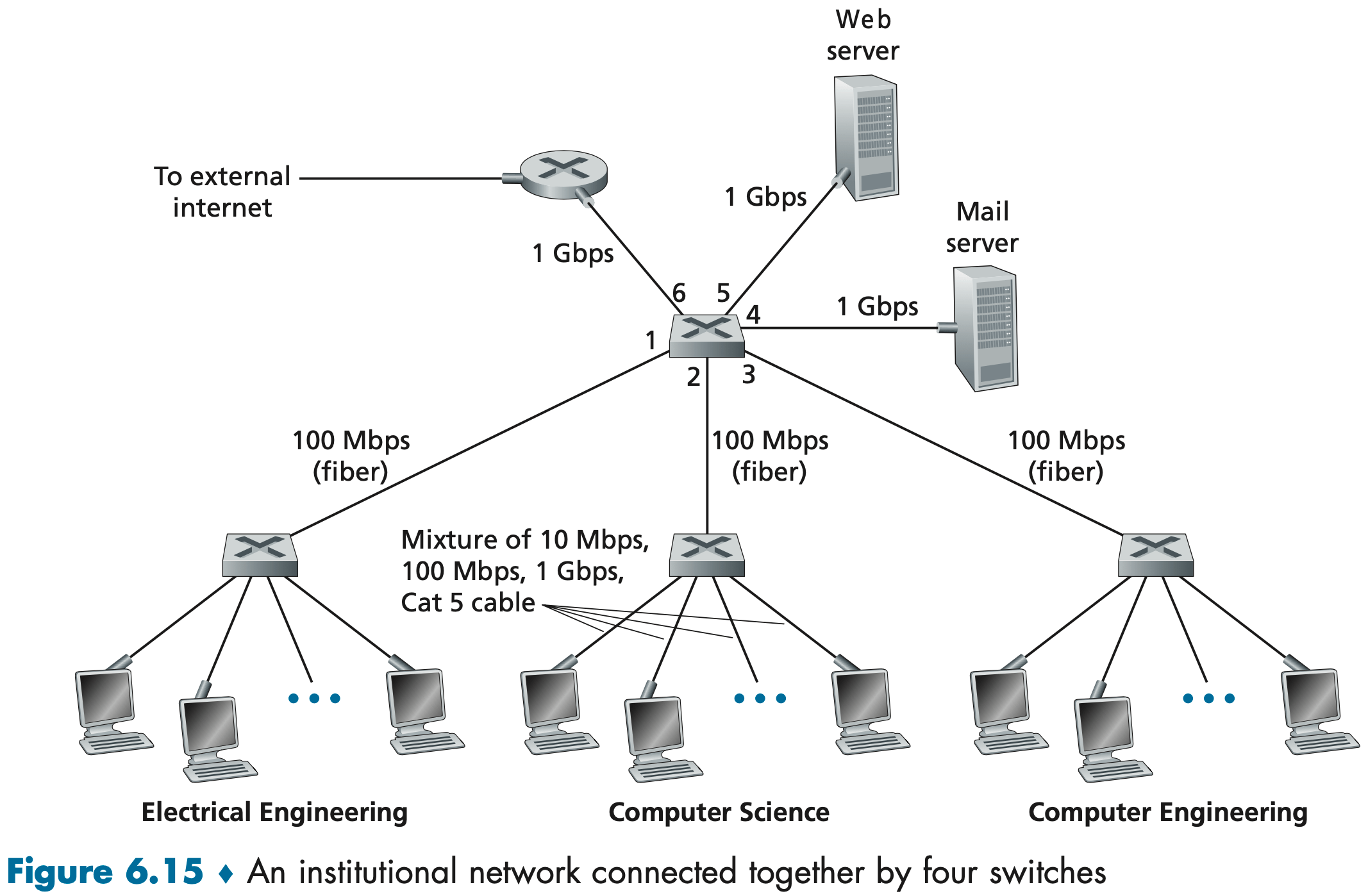
Figure 6.15 shows a switched local network connecting three departments, two servers and a router with four switches. Because these switches operate at the link layer, they switch link-layer frames (rather than network-layer datagrams), don’t recognize network-layer addresses, and don’t use routing algorithms like OSPF to determine paths through the network of layer-2 switches. Instead of using IP addresses, we will soon see that they use link-layer addresses to forward link-layer frames through the network of switches.

We’ll begin our study of switched LANs by first covering link-layer addressing. We then examine the celebrated Ethernet protocol. After examining link-layer addressing and Ethernet, we’ll look at how link-layer switches operate, and then see how these switches are often used to build large-scale LANs.

Link-Layer Addressing and ARP

In truth, it is not hosts and routers that have link-layer addresses but rather their adapters (that is, network interfaces) that have link-layer addresses. Link-layer switches do not have link-layer addresses associated with their interfaces that connect to hosts and routers. A link-layer address is variously called a LAN address, a physical address, or a MAC address. For most LANs (including Ethernet and 802.11 wireless LANs), the MAC address is 6 bytes long, giving 2 ^ 48 possible MAC addresses.

Although MAC addresses were designed to be permanent, it is now possible to change an adapter’s MAC address via software. For the rest of this section, however, we’ll assume that an adapter’s MAC address is fixed. One interesting property of MAC addresses is that no two adapters have the same address. The IEEE manages the MAC address space. In particular, when a company wants to manufacture adapters, it purchases a chunk of the address space consisting of 224 addresses for a nominal fee. IEEE allocates the chunk of 224 addresses by fixing the first 24 bits of a MAC address and letting the company create unique combinations of the last 24 bits for each adapter.

When an adapter wants to send a frame to some destination adapter, the sending adapter inserts the destination adapter’s MAC address into the frame and then sends the frame into the LAN. As we will soon see, a switch occasionally broadcasts an incoming frame onto all of its interfaces. 802.11 also broadcasts frames. Thus, an adapter may receive a frame that isn’t addressed to it. Thus, when an adapter receives a frame, it will check to see whether the destination MAC address in the frame matches its own MAC address. If there is a match, the adapter extracts the enclosed datagram and passes the datagram up the protocol stack. If there isn’t a match, the adapter discards the frame, without passing the network-layer datagram up.

However, sometimes a sending adapter does want all the other adapters on the LAN to receive and process the frame it is about to send. In this case, the sending adapter inserts a special MAC broadcast address into the destination address field of the frame. For LANs that use 6-byte addresses (such as Ethernet and 802.11), the broadcast address is a string of 48 consecutive 1s (that is, FF-FF-FF-FF-FF-FF in hexadecimal notation).

Because there are both network-layer addresses (for example, Internet IP addresses) and link-layer addresses (that is, MAC addresses), there is a need to translate between them. For the Internet, this is the job of the Address Resolution Protocol (ARP).

Each host and router has an ARP table in its memory, which contains mappings of IP addresses to MAC addresses. But what if the ARP table doesn’t currently have an entry for the destination? In this case, the sender uses the ARP protocol to resolve the address.

Ethernet

Today, Ethernet is by far the most prevalent wired LAN technology, and it is likely to remain so for the foreseeable future. One might say that Ethernet has been to local area networking what the Internet has been to global networking.

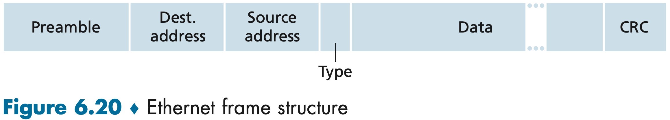
We can learn a lot about Ethernet by examining the Ethernet frame:

• Data field (46 to 1,500 bytes). This field carries the IP datagram. The maximum transmission unit (MTU) of Ethernet is 1,500 bytes. This means that if the IP datagram exceeds 1,500 bytes, then the host has to fragment the datagram, as discussed in Section 4.3.2. The minimum size of the data field is 46 bytes. This means that if the IP datagram is less than 46 bytes, the data field has to be “stuffed” to fill it out to 46 bytes. When stuffing is used, the data passed to the network layer contains the stuffing as well as an IP datagram. The network layer uses the length field in the IP datagram header to remove the stuffing.
• Destination address (6 bytes). This field contains the MAC address of the destination adapter. When destination adapter receives an Ethernet frame whose destination address is its or the MAC broadcast address, it passes the contents of the frame’s data field to the network layer; if it receives a frame with any other MAC address, it discards the frame.
• Source address (6 bytes). This field contains the MAC address of the adapter that transmits the frame onto the LAN.
• Type field (2 bytes). The type field permits Ethernet to multiplex network-layer protocols. To understand this, we need to keep in mind that hosts can use other network-layer protocols besides IP (e.g. ARP).
• Cyclic redundancy check (CRC) (4 bytes). As discussed in Section 6.2.3, the purpose of the CRC field is to allow the receiving adapter to detect bit errors in the frame.
• Preamble (8 bytes).

Many Ethernet technologies have been standardized over the years by the IEEE 802.3 CSMA/CD (Ethernet) working group. Ethernet is both a link-layer and a physical-layer specification and is carried over a variety of physical media including coaxial cable, copper wire, and fiber.

In a switch-based Ethernet LAN there are no collisions and, therefore, there is no need for a MAC protocol!

Link-Layer Switches

The role of the switch is to receive incoming link-layer frames and forward them onto outgoing links; we’ll study this forwarding function in detail in this subsection. We’ll see that the switch itself is transparent to the hosts and routers in the subnet; that is, a host/router addresses a frame to another host/router (rather than addressing the frame to the switch) and happily sends the frame into the LAN, unaware that a switch will be receiving the frame and forward- ing it.

Filtering is the switch function that determines whether a frame should be for- warded to some interface or should just be dropped. Forwarding is the switch function that determines the interfaces to which a frame should be directed, and then moves the frame to those interfaces. Switch filtering and forwarding are done with a switch table. As long as the switch table is complete and accurate, the switch forwards frames toward destinations without any broadcasting.

As we learned in Chapter 4, routers are store-and-forward packet switches that for- ward packets using network-layer addresses. Although a switch is also a store-and- forward packet switch, it is fundamentally different from a router in that it forwards packets using MAC addresses. Whereas a router is a layer-3 packet switch, a switch is a layer-2 packet switch. Recall, however, that we learned in Section 4.4 that mod- ern switches using the “match plus action” operation can be used to forward a layer-2 frame based on the frame's destination MAC address, as well as a layer-3 datagram using the datagram's destination IP address. Indeed, we saw that switches using the OpenFlow standard can perform generalized packet forwarding based on any of eleven different frame, datagram, and transport-layer header fields.

Even though switches and routers are fundamentally different, network admin- istrators must often choose between them when installing an interconnection device. What are the pros and cons of the two approaches?

First consider the pros and cons of switches. As mentioned above, switches are plug-and-play, a property that is cherished by all the overworked network adminis- trators of the world. Switches can also have relatively high filtering and forwarding rates—as shown in Figure 6.24, switches have to process frames only up through layer 2, whereas routers have to process datagrams up through layer 3. On the other hand, to prevent the cycling of broadcast frames, the active topology of a switched network is restricted to a spanning tree. Also, a large switched network would require large ARP tables in the hosts and routers and would generate substantial ARP traffic and processing. Furthermore, switches are susceptible to broadcast storms—if one host goes haywire and transmits an endless stream of Ethernet broadcast frames, the switches will forward all of these frames, causing the entire network to collapse.

Now consider the pros and cons of routers. Because network addressing is often hierarchical (and not flat, as is MAC addressing), packets do not normally cycle through routers even when the network has redundant paths. (However, packets can cycle when router tables are misconfigured; but as we learned in Chapter 4, IP uses a special datagram header field to limit the cycling.) Thus, packets are not restricted to a spanning tree and can use the best path between source and destination. Because routers do not have the spanning tree restriction, they have allowed the Internet to be built with a rich topology that includes, for example, multiple active links between Europe and North America. Another feature of routers is that they provide firewall protection against layer-2 broadcast storms. Perhaps the most significant drawback of routers, though, is that they are not plug-and-play—they and the hosts that connect to them need their IP addresses to be configured. Also, routers often have a larger per-packet processing time than switches, because they have to process up through the layer-3 fields.

A Day in the Life of a Web Page Request

A student, Bob, connects his laptop to an Ethernet cable connected to the school’s Ethernet switch and downloads a Web page.

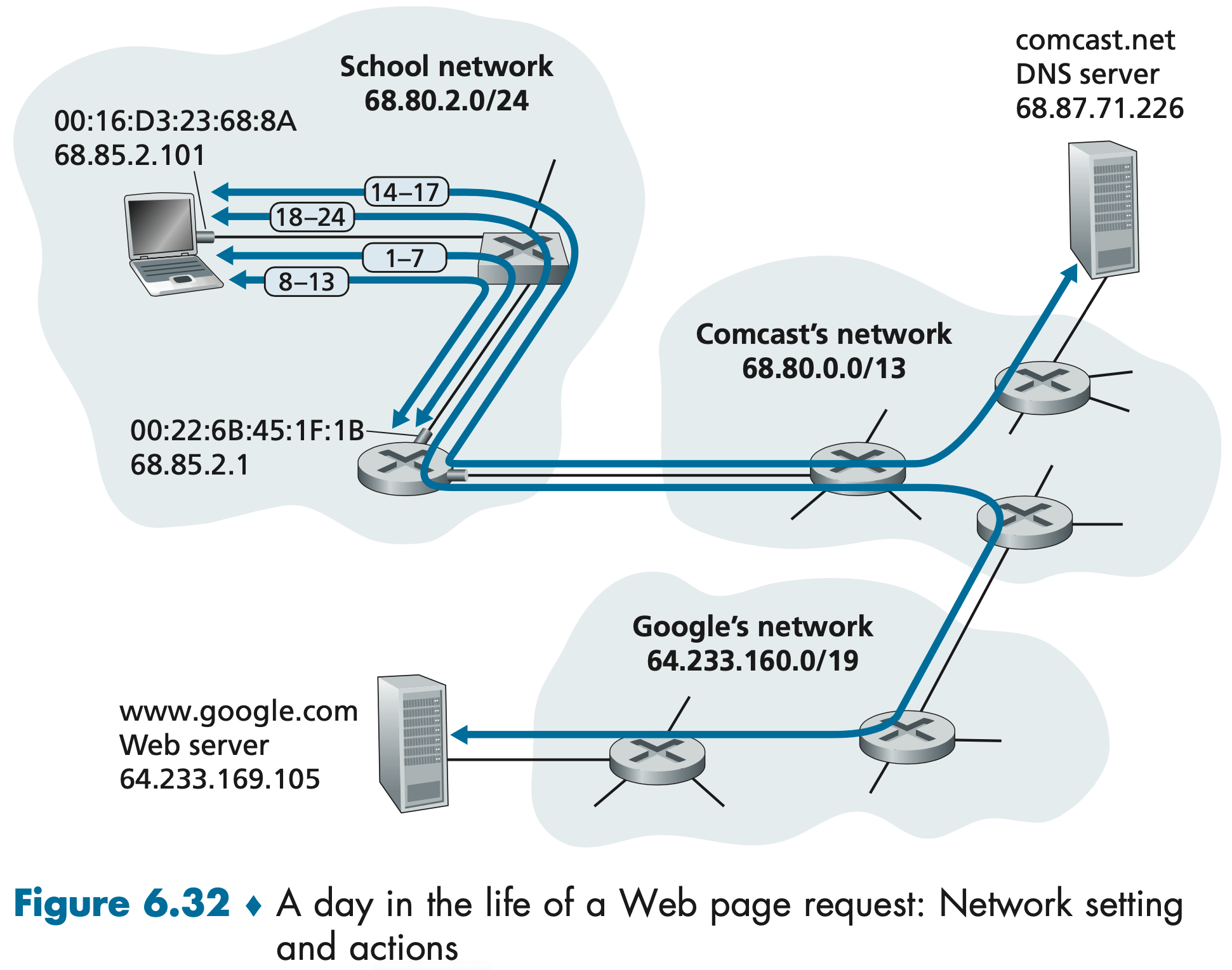
1. The operating system on Bob’s laptop creates a DHCP request message (Section 4.3.3) and puts this message within a UDP segment (Section 3.3) with destination port 67 (DHCP server) and source port 68 (DHCP client). The UDP segment is then placed within an IP datagram (Section 4.3.1) with a broadcast IP destination address (255.255.255.255) and a source IP address of 0.0.0.0, since Bob’s laptop doesn’t yet have an IP address.
2. The IP datagram containing the DHCP request message is then placed within an Ethernet frame (Section 6.4.2). The Ethernet frame has a destination MAC addresses of FF:FF:FF:FF:FF:FF so that the frame will be broadcast to all devices connected to the switch (hopefully including a DHCP server); the frame’s source MAC address is that of Bob’s laptop, 00:16:D3:23:68:8A.
3. The broadcast Ethernet frame containing the DHCP request is the first frame sent by Bob’s laptop to the Ethernet switch. The switch broadcasts the incoming frame on all outgoing ports, including the port connected to the router.
4. The router receives the broadcast Ethernet frame containing the DHCP request on its interface with MAC address 00:22:6B:45:1F:1B and the IP datagram is extracted from the Ethernet frame. The datagram’s broadcast IP destination address indicates that this IP datagram should be processed by upper layer protocols at this node, so the datagram’s payload (a UDP segment) is thus demultiplexed (Section 3.2) up to UDP, and the DHCP request message is extracted from the UDP segment. The DHCP server now has the DHCP request message.
5. Let’s suppose that the DHCP server running within the router can allocate IP addresses in the CIDR (Section 4.3.3) block 68.85.2.0/24. In this example, all IP addresses used within the school are thus within Comcast’s address block. Let’s suppose the DHCP server allocates address 68.85.2.101 to Bob’s laptop. The DHCP server creates a DHCP ACK message (Section 4.3.3) containing this IP address, as well as the IP address of the DNS server (68.87.71.226), the IP address for the default gateway router (68.85.2.1), and the subnet block (68.85.2.0/24) (equivalently, the “network mask”). The DHCP message is put inside a UDP segment, which is put inside an IP datagram, which is put inside an Ethernet frame. The Ethernet frame has a source MAC address of the router’s interface to the home network (00:22:6B:45:1F:1B) and a destination MAC address of Bob’s laptop (00:16:D3:23:68:8A).
6. The Ethernet frame containing the DHCP ACK is sent (unicast) by the router to the switch. Because the switch is self-learning (Section 6.4.3) and previously received an Ethernet frame (containing the DHCP request) from Bob’s laptop, the switch knows to forward a frame addressed to 00:16:D3:23:68:8A only to the output port leading to Bob’s laptop.
7. Bob’s laptop receives the Ethernet frame containing the DHCP ACK, extracts the IP datagram from the Ethernet frame, extracts the UDP segment from the IP datagram, and extracts the DHCP ACK message from the UDP segment. Bob’s DHCP client then records its IP address and the IP address of its DNS server. It also installs the address of the default gateway into its IP forward- ing table (Section 4.1). Bob’s laptop will send all datagrams with destination address outside of its subnet 68.85.2.0/24 to the default gateway. At this point, Bob’s laptop has initialized its networking components and is ready to begin processing the Web page fetch.
8. The operating system on Bob’s laptop thus creates a DNS query message (Section 2.5.3), putting the string "www.google.com" in the question section of the DNS message. This DNS message is then placed within a UDP segment with a destination port of 53 (DNS server). The UDP segment is then placed within an IP datagram with an IP destination address of 68.87.71.226 (the address of the DNS server returned in the DHCP ACK in step 5) and a source IP address of 68.85.2.101.
9. Bob’s laptop then places the datagram containing the DNS query message in an Ethernet frame. This frame will be sent (addressed, at the link layer) to the gateway router in Bob’s school’s network. However, even though Bob’s laptop knows the IP address of the school’s gateway router (68.85.2.1) via the DHCP ACK message in step 5 above, it doesn’t know the gateway router’s MAC address. In order to obtain the MAC address of the gateway router, Bob’s laptop will need to use the ARP protocol (Section 6.4.1).
10. Bob’s laptop creates an ARP query message with a target IP address of 68.85.2.1 (the default gateway), places the ARP message within an Ethernet frame with a broadcast destination address (FF:FF:FF:FF:FF:FF) and sends the Ethernet frame to the switch, which delivers the frame to all connected devices, including the gateway router.
11. ThegatewayrouterreceivestheframecontainingtheARPquerymessageonthe interface to the school network, and finds that the target IP address of 68.85.2.1 in the ARP message matches the IP address of its interface. The gateway router thus prepares an ARP reply, indicating that its MAC address of 00:22:6B:45:1F:1B corresponds to IP address 68.85.2.1. It places the ARP reply message in an Ethernet frame, with a destination address of 00:16:D3:23:68:8A (Bob’s laptop) and sends the frame to the switch, which delivers the frame to Bob’s laptop.
12. Bob’s laptop receives the frame containing the ARP reply message and extracts the MAC address of the gateway router (00:22:6B:45:1F:1B) from the ARP reply message.
13. Bob’s laptop can now (finally!) address the Ethernet frame containing the DNS query to the gateway router’s MAC address. Note that the IP datagram in this frame has an IP destination address of 68.87.71.226 (the DNS server), while the frame has a destination address of 00:22:6B:45:1F:1B (the gateway router). Bob’s laptop sends this frame to the switch, which delivers the frame to the gateway router.
14. The gateway router receives the frame and extracts the IP datagram containing the DNS query. The router looks up the destination address of this datagram (68.87.71.226) and determines from its forwarding table that the datagram should be sent to the leftmost router in the Comcast network in Figure 6.32. The IP datagram is placed inside a link-layer frame appropriate for the link connecting the school’s router to the leftmost Comcast router and the frame is sent over this link.
15. The leftmost router in the Comcast network receives the frame, extracts the IP datagram, examines the datagram’s destination address (68.87.71.226) and determines the outgoing interface on which to forward the datagram toward the DNS server from its forwarding table, which has been filled in by Comcast’s intra-domain protocol (such as RIP, OSPF or IS-IS, Section 5.3) as well as the Internet’s inter-domain protocol, BGP (Section 5.4).
16. Eventually the IP datagram containing the DNS query arrives at the DNS server. The DNS server extracts the DNS query message, looks up the name www.google.com in its DNS database (Section 2.5), and finds the DNS resource record that contains the IP address (64.233.169.105) for www.google.com. (assuming that it is currently cached in the DNS server). Recall that this cached data originated in the authoritative DNS server (Section 2.5.2) for google.com. The DNS server forms a DNS reply message containing this hostname-to-IP-address mapping, and places the DNS reply message in a UDP segment, and the segment within an IP datagram addressed to Bob’s laptop (68.85.2.101). This datagram will be forwarded back through the Comcast network to the school’s router and from there, via the Ethernet switch to Bob’s laptop.
17. Bob’s laptop extracts the IP address of the server www.google.com from the DNS message. Finally, after a lot of work, Bob’s laptop is now ready to contact the www.google.com server!
18. Now that Bob’s laptop has the IP address of www.google.com, it can create the TCP socket (Section 2.7) that will be used to send the HTTP GET message (Section 2.2.3) to www.google.com. When Bob creates the TCP socket, the TCP in Bob’s laptop must first perform a three-way handshake (Section 3.5.6) with the TCP in www.google.com. Bob’s laptop thus first creates a TCP SYN segment with destination port 80 (for HTTP), places the TCP segment inside an IP datagram with a destination IP address of 64.233.169.105 (www.google.com), places the datagram inside a frame with a destination MAC address of 00:22:6B:45:1F:1B (the gateway router) and sends the frame to the switch.
19. The routers in the school network, Comcast’s network, and Google’s network forward the datagram containing the TCP SYN toward www.google.com, using the forwarding table in each router, as in steps 14–16 above. Recall that the router forwarding table entries governing forwarding of packets over the inter-domain link between the Comcast and Google networks are determined by the BGP protocol (Chapter 5).
20. Eventually, the datagram containing the TCP SYN arrives atwww.google.com. The TCP SYN message is extracted from the datagram and demultiplexed to the welcome socket associated with port 80. A connection socket (Section 2.7) is created for the TCP connection between the Google HTTP server and Bob’s laptop. A TCP SYNACK (Section 3.5.6) segment is generated, placed inside a datagram addressed to Bob’s laptop, and finally placed inside a link-layer frame appropriate for the link connecting www.google.com to its first-hop router.
21. The datagram containing the TCP SYNACK segment is forwarded through the Google, Comcast, and school networks, eventually arriving at the Ethernet controller in Bob’s laptop. The datagram is demultiplexed within the operating system to the TCP socket created in step 18, which enters the connected state.
22. With the socket on Bob’s laptop now (finally!) ready to send bytes to www.google.com, Bob’s browser creates the HTTP GET message (Section 2.2.3) containing the URL to be fetched. The HTTP GET message is then written into the socket, with the GET message becoming the payload of a TCP segment. The TCP segment is placed in a datagram and sent and delivered to www.google.com as in steps 18–20 above.
23. The HTTP server at www.google.com reads the HTTP GET message from the TCP socket, creates an HTTP response message (Section 2.2), places the requested Web page content in the body of the HTTP response message, and sends the message into the TCP socket.
24. The datagram containing the HTTP reply message is forwarded through the Google, Comcast, and school networks, and arrives at Bob’s laptop. Bob’s Web browser program reads the HTTP response from the socket, extracts the html for the Web page from the body of the HTTP response, and finally (finally!) displays the Web page!

Wireless and Mobile Networks

A base station is responsible for sending and receiving data (e.g., packets) to and from a wireless host that is associated with that base station. Cell towers in cellular networks and access points in 802.11 wireless LANs are examples of base stations.

When a mobile host moves beyond the range of one base station and into the range of another—a process referred to as handoff or handover.

At the highest level we can classify wireless networks to:

• Single-hop, infrastructure-based. These networks have a base station that is connected to a larger wired network (e.g., the Internet). Furthermore, all communication is between this base station and a wireless host over a single wireless hop. The 802.11 networks you use in the classroom, café, or library; and the 4G LTE data networks all fall in this category.
• Single-hop, infrastructure-less. In these networks, there is no base station that is connected to a wireless network. However, as we will see, one of the nodes in this single-hop network may coordinate the transmissions of the other nodes. Bluetooth networks fall in this.
• Multi-hop, infrastructure-based. In these networks, a base station is present that is wired to the larger network. However, some wireless nodes may have to relay their communication through other wireless nodes in order to communicate via the base station. Some wireless sensor networks and so-called wireless mesh networks deployed in homes fall in this category.
• Multi-hop, infrastructure-less. There is no base station in these networks, and nodes may have to relay messages among several other nodes in order to reach a destination. Nodes may also be mobile, with connectivity changing among nodes—a class of networks known as mobile ad hoc networks (MANETs). If the mobile nodes are vehicles, the network is a vehicular ad hoc network (VANET). As you might imagine, the development of protocols for such net- works is challenging and is the subject of much ongoing research.

Bluetooth operates over short ranges, at low power, and at low cost. Bluetooth networks operate in the unlicensed 2.4 GHz radio band. The Bluetooth wireless channel is operated in a TDM manner, with time slots of 625 microseconds. Bluetooth data rates can reach up to 3 Mbps.

Bluetooth networks are ad hoc networks. Bluetooth devices must organize themselves into a piconet of up to eight active devices. One of these devices is designated as the master, with the remaining devices acting as clients. In addition to the active devices, there can also be up to 255 “parked” devices in the piconet. These parked devices are often in some form of “sleep mode” to conserve energy and will awaken periodically, according to the master’s schedule, to receive beacon messages from the master. A parked device cannot communicate until its status has been changed from parked to active by the master node.

Wireless Links and WiFi

Wireless links differ from their wired counterparts in a number important ways: Decreasing signal strength; Interference from other sources; Multipath propagation. Bit errors will be more common in wireless links than in wired links. For this reason, wireless link protocols employ not only powerful CRC error detection codes, but also link-level reliable-data-transfer protocols that retransmit corrupted frames.

This host receives an electromagnetic signal that is a combination of a degraded form of the original signal transmitted by the sender (degraded due to the attenuation and multipath propagation effects that we discussed above, among others) and background noise in the environment. The signal-to-noise ratio (SNR) is a relative measure of the strength of the received signal and this noise. The SNR is typically measured in units of decibels (dB). A larger SNR makes it easier for the receiver to extract the transmitted signal from the background noise.

Although many technologies and standards for wireless LANs were developed in the 1990s, one particular class of standards has clearly emerged as the winner: the IEEE 802.11 wireless LAN, also known as WiFi.

The fundamental building block of the 802.11 architecture is the basic service set (BSS). A BSS contains one or more wireless stations and a central base station, known as an access point (AP) in 802.11 parlance. As with Ethernet devices, each 802.11 wireless station has a 6-byte MAC address that is stored in the firmware of the station’s adapter (that is, 802.11 network interface card). Each AP also has a MAC address for its wireless interface. As with Ethernet, these MAC addresses are administered by IEEE and are (in theory) globally unique.

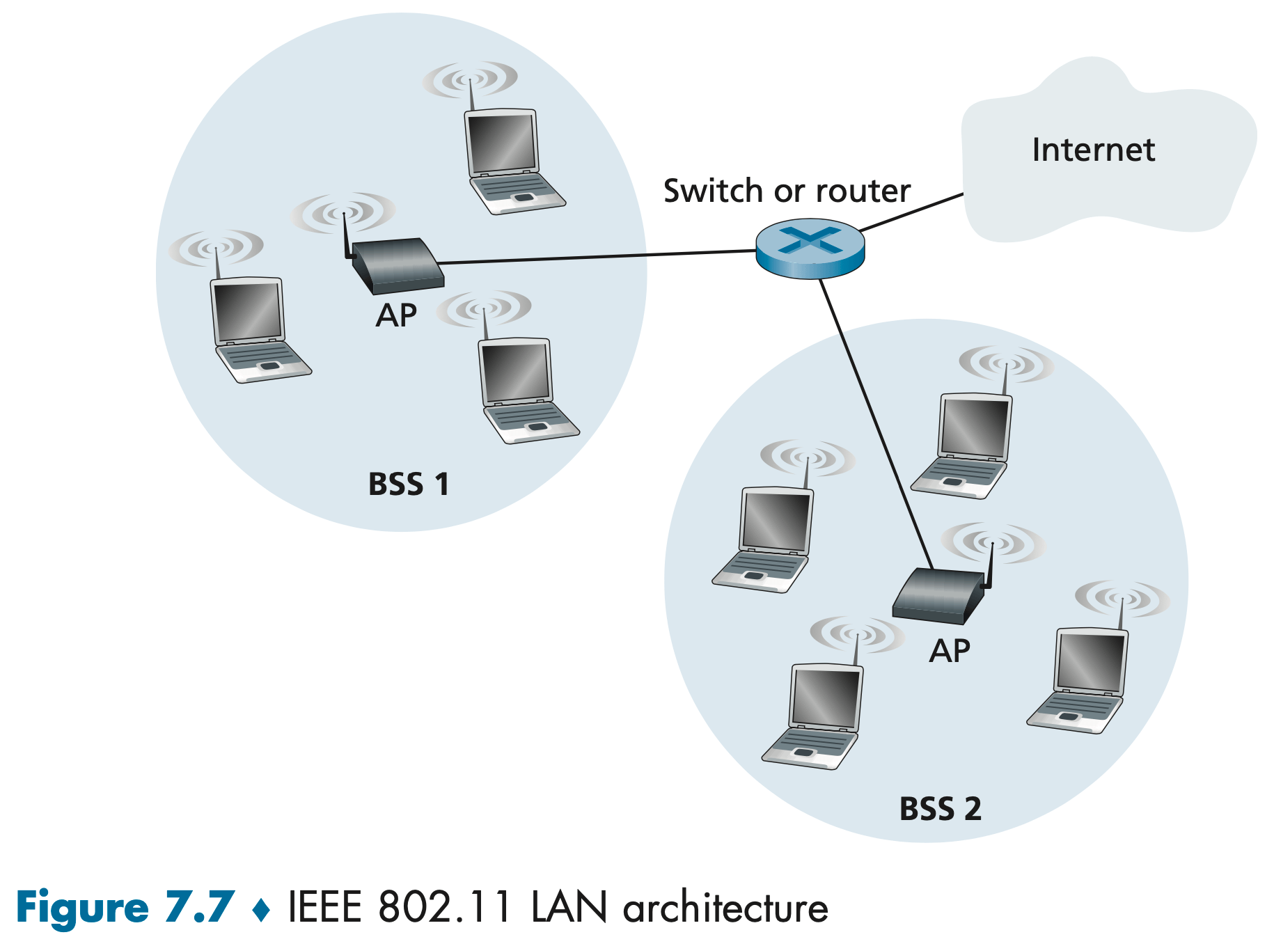
When a network administrator installs an AP, the administrator assigns a one- or two-word Service Set Identifier (SSID) to the access point（即 Wi-Fi 列表里显示的名称）. The 802.11 standard requires that an AP periodically send beacon frames, each of which includes the AP’s SSID and MAC address.

The process of scanning channels and listening for beacon frames is known as passive scanning. A wireless device can also perform active scanning, by broadcasting a probe frame that will be received by all APs within the wireless device’s range.

In order to create an association with a particular AP, the wireless device may be required to authenticate itself to the AP. One approach is to permit access based on a device’s MAC address. A second approach employs usernames and passwords.

Because multiple wireless devices, or the AP itself may want to transmit data frames at the same time over the same channel, a multiple access protocol is needed to coordinate the transmissions. Inspired by the huge success of Ethernet and its random access protocol, the designers of 802.11 chose CSMA with collision avoidance (CSMA/CA). 802.11 uses collision-avoidance techniques and link-layer acknowledgment/retransmission (ARQ) scheme.

Mobility in the Same IP Subnet

In order to increase the physical range of a wireless LAN, companies and universities will often deploy multiple BSSs within the same IP subnet. This naturally raises the issue of mobility among the BSSs—how do wireless stations seamlessly move from one BSS to another while maintaining ongoing TCP sessions?

Mobility can be handled in a relatively straightforward manner when the BSSs are part of the subnet.

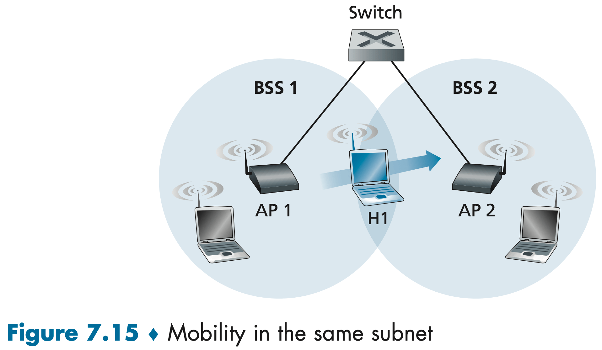
Figure 7.15 shows two interconnected BSSs with a host, H1, moving from BSS1 to BSS2. Because in this example the interconnection device that connects the two BSSs is not a router, all of the stations in the two BSSs, including the APs, belong to the same IP subnet. Thus, when H1 moves from BSS1 to BSS2, it may keep its IP address and all of its ongoing TCP connections. If the interconnection device were a router, then H1 would have to obtain a new IP address in the subnet in which it was moving. This address change would disrupt (and eventually terminate) any on-going TCP connections at H1. In Section 7.6, we’ll see how a network-layer mobility protocol, such as mobile IP, can be used to avoid this problem.

As H1 wanders away from AP1, H1 detects a weakening signal from AP1 and starts to scan for a stronger signal. H1 receives beacon frames from AP2 (which in many corporate and university settings will have the same SSID as AP1). H1 then disassociates with AP1 and associates with AP2, while keeping its IP address and maintaining its ongoing TCP sessions.

But what about the switch? How does it know that the host has moved from one AP to another? As you may recall from Chapter 6, switches are “self-learning” and automatically build their forwarding tables. This self-learning feature nicely handles occasional moves; however, switches were not designed to support highly mobile users who want to maintain TCP connections while moving between BSSs. To appreciate the problem here, recall that before the move, the switch has an entry in its forwarding table that pairs H1’s MAC address with the outgoing switch interface through which H1 can be reached. If H1 is initially in BSS1, then a datagram destined to H1 will be directed to H1 via AP1. Once H1 associates with BSS2, however, its frames should be directed to AP2. One solution (a bit of a hack, really) is for AP2 to send a broadcast Ethernet frame with H1’s source address to the switch just after he new association. When the switch receives the frame, it updates its forwarding table, allowing H1 to be reached via AP2. The 802.11f standards group is developing an inter-AP protocol to handle these and related issues.

Cellular Networks: 4G and 5G

In a relatively short span of 20 years, cellular carrier networks have undergone an astonishing transition from being almost exclusively circuit-switched telephone networks to being all-IP packet-switched data networks.

The term cellular refers to the fact that the region covered by a cellular network is partitioned into a number of geographic coverage areas, known as cells. Each cell contains a base station that transmits signals to, and receives signals from, the mobile devices currently in its cell.

The 4G networks that are pervasive implement the 4G Long-Term Evolution standard, or more succinctly 4G LTE.

The mobile device is a network endpoint, with an IP address (obtained through NAT). The mobile device also has a globally unique 64-bit identifier called the International Mobile Subscriber Identity (IMSI), which is stored on its SIM (Subscriber Identity Module) card.

LTE Element	Description	Similar WLAN function(s)
Mobile device	End user’s IP-capable wireless/mobile device	Host, end-system
Base Station	Network side of wireless access link into LTE network	Access point (AP), although the LTE base station performs many functions not found in WLANs
The Mobility Management Entity (MME)	Coordinator for mobile device services: authentication, mobility management	Access point (AP), although the MME performs many functions not found in WLANs
Home Subscriber Server (HSS)	Located in a mobile device’s home network, providing authentication, access privileges in home and visited networks	No WLAN equivalent
Serving Gateway (S-GW), PDN-Gateway (P-GW)	Routers in a cellular carrier’s network, coordinating forwarding to outside of the carrier’s network	iBGP and eBGP routers in access ISP network
Radio Access Network	Wireless link between mobile device and a base station	802.11 wireless link between mobile and AP

LTE uses a combination of frequency division multiplexing and time division multi- plexing on the downstream channel, known as orthogonal frequency division multi- plexing (OFDM).（频分复用和时分复用结合，称为正交频分复用）

The ultimate wide-area data service would be one with ubiquitous gigabit connec- tion speeds, extremely low latency, and unrestricted limitations on the number of users and devices that could be supported in any region. It is expected that 5G, for which progressively improved versions are likely to be rolled out in the 2020 decade, will make a big step towards achieving the goals of the ultimate wide-area data service.

5G standards divide frequencies into two groups: FR1 (450 MHz–6 GHz) and FR2 (24 GHz–52 GHz). FR2 frequencies are also known as millimeter wave frequencies. Many 5G innovations will be a direct result of working in the millimeter wave fre- quencies in the 24 GHz–52 GHz band.

5G is expected to provide a 100x increase in capacity in urban areas. Similarly, owing to the much wider fre- quency band, 5G is expected to provide peak download rates of 1 Gbps or higher. Millimeter wave signals are, however, easily blocked by buildings and trees. Small cell stations are needed to fill in coverage gaps between base stations and users. In a highly populous region, the distance between two small cells could vary from 10 to 100 meters.

Network Security

Network Under Attack

Much of the malware out there today is self-replicating: once it infects one host, from that host it seeks entry into other hosts over the Internet, and from the newly infected hosts, it seeks entry into yet more hosts. Malware can spread in the form of a virus or a worm. Viruses are malware that require some form of user interaction to infect the user’s device. Worms are malware that can enter a device without any explicit user interaction.

Another broad class of security threats are known as denial-of-service (DoS) attacks. As the name suggests, a DoS attack renders a network, host, or other piece of infrastructure unusable by legitimate users.

A passive receiver that records a copy of every packet that flies by is called a packet sniffer.

It is surprisingly easy to create a packet with an arbitrary source address, packet content, and destination address and then transmit this hand-crafted packet into the Internet, which will dutifully forward the packet to its destination. Imagine the unsuspecting receiver (say an Internet router) who receives such a packet, takes the (false) source address as being truthful, and then performs some command embedded in the packet’s contents (say modifies its forwarding table). The ability to inject packets into the Internet with a false source address is known as IP spoofing, and is but one of many ways in which one user can masquerade as another user.

Symmetric Key Cryptography

Prefer: AES-GCM, ChaCha20/Poly1305.

Deprecated: RC4, 3DES-CBC, AES-CBC.

Public Key Encryption

Prefer: >= 2048-bit RSA, Elliptic Curves

Cryptographic Hash Functions

Prefer: SHA-2 Family.

Deprecated: MD5, SHA-1.

Digital Signatures

An important application of digital signatures is public key certification, that is, certifying that a public key belongs to a specific entity.

Transport Layer Security (TLS)

Desirable properties of secure communication (Transport layer security provides):

• Encryption: So it can’t be read by other people.
• Integrity: The message can’t be altered without detection.
• Authentication: Prove the identity of exactly who you are talking to.

TLS is often used to provide security to transactions that take place over HTTP. However, because TLS secures TCP, it can be employed by any application that runs over TCP. TLS provides a simple Application Programmer Interface (API) with sockets, which is similar and analogous to TCP’s API.

TLS has three phases: handshake, key derivation, and data transfer. We now describe these three phases for a communication session between a client (Bob) and a server (Alice), with Alice having a private/public key pair and a certificate that binds her identity to her public key.

1. Once the TCP connection is established, Bob sends Alice a hello message. The client sends a list of cryptographic algorithms it supports, along with a client nonce.
2. From the list, the server chooses a symmetric algorithm (for example, AES) and a public key algorithm (for example, RSA with a specific key length), and HMAC algorithm (MD5 or SHA-1) along with the HMAC keys. It sends back to the client its choices, as well as a certificate and a server nonce.
3. Because the certificate has been certified by a CA, Bob knows for sure that the public key in the certificate belongs to Alice. Bob generates a Pre-Master Secret (PMS), encrypts the PMS with the server’s public key, and sends the encrypted PMS to the server. The client sends the HMAC of all the handshake messages.
4. Using the same key derivation function (as specified by the TLS standard), the client and server independently compute the Master Secret (MS) from the PMS and nonces. The MS is then sliced up to generate the two encryption and two HMAC keys. HMAC is a standardized hashed message authentication code (MAC). Henceforth, all messages sent between client and server are encrypted and authenticated (with the HMAC). The server sends the HMAC of all the handshake messages.

Four keys:

• EB = session encryption key for data sent from Bob to Alice
• MB = session HMAC key for data sent from Bob to Alice
• EA = session encryption key for data sent from Alice to Bob
• MA = session HMAC key for data sent from Alice to Bob

Now that Alice and Bob share the same four session keys (EB, MB, EA, and MA), they can start to send secured data to each other over the TCP connection. Since TCP is a byte-stream protocol, TLS breaks the data stream into records, appends an HMAC to each record for integrity checking, and then encrypts the record+HMAC. This encrypted package is then passed to TCP for transport over the Internet.

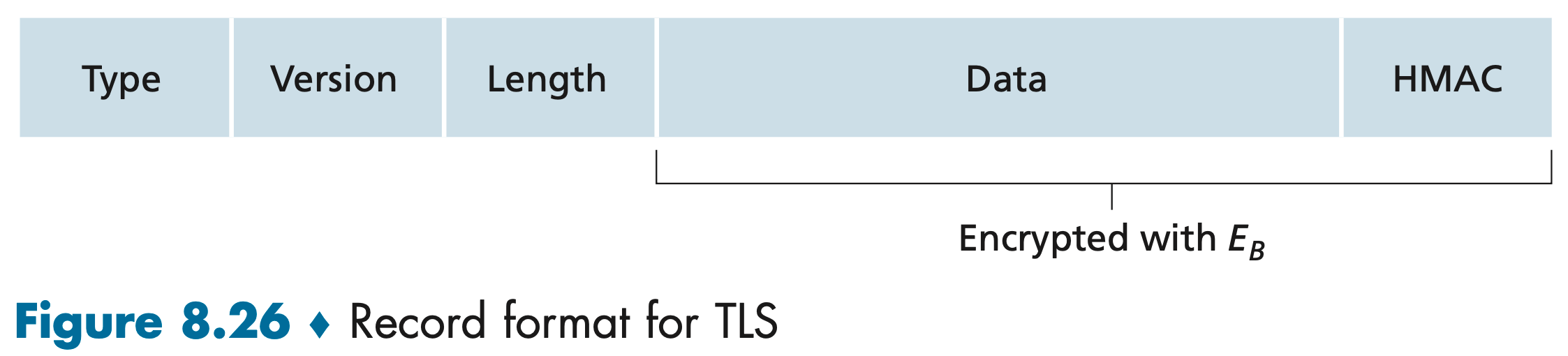
Bob maintains a sequence number counter, which begins at zero and is incremented for each TLS record he sends. Bob doesn’t actually include a sequence number in the record itself, but when he calculates the HMAC, he includes the sequence number in the HMAC calculation. Thus, the HMAC is now a hash of the data plus the HMAC key plus the current sequence number. Alice tracks Bob’s sequence numbers, allowing her to verify the data integrity of a record by including the appropriate sequence number in the HMAC calculation. This use of TLS sequence numbers prevents Trudy from carrying out a woman-in-the-middle attack, such as reordering or replaying segments.

You may be wondering why there are nonces in steps 1 and 2. Don’t sequence numbers suffice for preventing the segment replay attack? The answer is yes, but they don’t alone prevent the “connection replay attack.” Suppose Trudy sniffs all messages between Alice and Bob. The next day, Trudy masquerades as Bob and sends to Alice exactly the same sequence of messages that Bob sent to Alice on the previous day. If Alice doesn’t use nonces, she will respond with exactly the same sequence of messages she sent the previous day. Alice will not suspect any funny business, as each message she receives will pass the integrity check. If Alice is an e-commerce server, she will think that Bob is placing a second order (for exactly the same thing). On the other hand, by including a nonce in the protocol, Alice will send different nonces for each TCP session, causing the encryption keys to be different on the two days. Therefore, when Alice receives played-back TLS records from Trudy, the records will fail the integrity checks, and the bogus e-commerce transaction will not succeed. In summary, in TLS, nonces are used to defend against the “connection replay attack” and sequence numbers are used to defend against replaying individual packets during an ongoing session.

At some point, either Bob or Alice will want to end the TLS session. One approach would be to let Bob end the TLS session by simply terminating the underlying TCP connection. But such a naive design sets the stage for the truncation attack. If Trudy were to do this, Alice would think she received all of Bob’s data when actuality she only received a portion of it.

The solution to this problem is to indicate in the type field whether the record serves to terminate the TLS session. (Although the TLS type is sent in the clear, it is authenticated at the receiver using the record’s HMAC.) By including such a field, if Alice were to receive a TCP FIN before receiving a closure TLS record, she would know that something funny was going on.

HTTPS 详解一：附带最精美详尽的 HTTPS 原理图

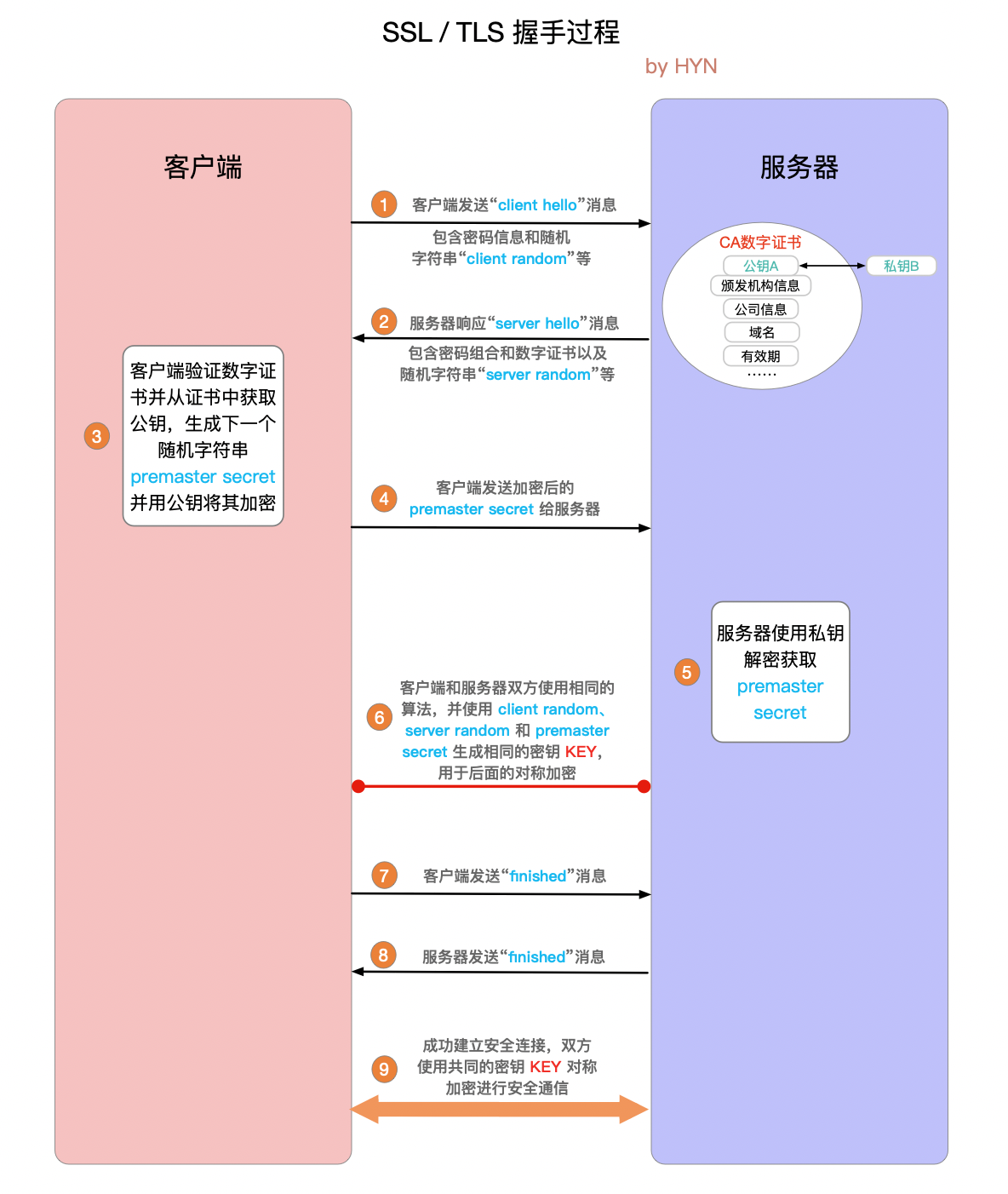
IPsec and VPNs

The IP security protocol, more commonly known as IPsec, provides security at the network layer. IPsec secures IP datagrams between any two network-layer entities, including hosts and routers.

An institution that extends over multiple geographical regions often desires its own IP network, so that its hosts and servers can send data to each other in a secure and confidential manner. To achieve this goal, the institution could actually deploy a stand-alone physical network, called a private network.

Instead of deploying and maintaining a private network, many institutions today create VPNs over the existing public Internet. With a VPN, the institution’s inter-office traffic is sent over the public Internet rather than over a physically independent network.

We'll focus on the Encapsulation Security Payload (ESP) protocol in the IPsec protocol suite. The ESP protocol provides source authentication, data integrity, and confidentiality.

Before sending IPsec datagrams from source entity to destination entity, the source and destination entities create a network-layer logical connection. This logical connection is called a security association (SA). An SA is unidirectional, if both entities want to send secure datagrams to each other, then two SAs need to be established.

Large, geographically distributed deployments require an automated mechanism for creating the SAs. IPsec does this with the Internet Key Exchange (IKE) protocol.